


 text new page (beta)
 English (pdf)
 Article in xml format
 Article references
 Send this article by e-mail
 Cited by SciELO
  Similars in
SciELO
Similars in
SciELO 
 Permalink
INTRODUCTION
The proposal is to study the scope of impact that high levels of air pollution have in the economy and competitiveness of the population in Mexicali, derived from health impact. In order to achieve this, the costs attributed to public health benefits (PHB) are estimated by establishing scenarios in the reduction of particulate matter equal or smaller than 10 micrometers in aerodynamic diameter (PM10), one of the main air pollutants in the city of Mexicali. In fact, the World Health Organization (WHO) has recently indicated that Mexicali is considered the 4th most polluted city in the world (WHO 2011, MEBC 2012) due to particulate matter equal or smaller than 2.5 micrometers in aerodynamic diameter (PM2.5), despite the fact that the National Institute of Ecology and Climate Change (INECC for its acronym in spanish) had previously warned about the serious pollution problem that this city shows (Zuk 2007).
In order to estimate the PHB, the method employed is "health impact assessment (HIA)", using as a guide the proposal presented by the INECC (2011).
To estimate the economic impact of air pollution, the potential benefits (impacts that could be avoided) that could be achieved in health (i.e. PHB) were the first to measure, due to the action of reducing the level concentration of the air pollutant considered in this study (i.e. PM10). Then, the estimated PHB was economically assessed by the human capital approach for mortality and the cost of illness (CoI) approach for morbidity.
Several studies show that PM10 can be used as a causal pollutant (Schwartz 1992, Ostro 1993, Schwartz 1993, WHO 1996), besides the fact of being a good indicator for the presence of other air pollutants (i.e. a combination of particles from different sources). Therefore, the PHB estimated by PM10 will be understood as being a consequence of the causal relationship between the total mix of this pollutant and their impacts in local health.
Even though the WHO states that all the effects on health as a consequence of the exposure to air pollution are important, it is not practical to include them all in a HIA (WHO 2000). The health impacts considered in this study were selected based on the local data available and on the recommendations made in a forum of experts on binational surveillance of diseases related to air pollution, coordinated by the Universidad Autónoma de Baja California-Mexicali in May 18th, 2006 (SDSU-UABC 2006). The best indicators that would help to measure the effects of air pollution on the local human population were defined. Therefore, the health impacts assessed in this document are: 1) mortality, 2) emergency room visits due to asthma (J45 in ICD-10 codes) and asthmatic status (J46 in ICD-10 codes), 3) hospitalizations due to asthma and asthmatic status, and 4) restricted activity days (RAD).
The aim of this study was to assess, as a first approach, the benefits in terms of Public Health (i.e. PHB for avoided cases) attributable to different PM10 reduction scenarios in Mexicali, Baja California, Mexico.
MATERIALS AND METHODS
To achieve the estimation of the avoided health impacts during the 2013 to 2020 period, data projected by the authors is used from these years. The projections for each variable were made based on their trend, using linear regression models for population projections and linear or nonlinear regression models for other variables which best suit (R2) the historical data for years previous to 2013.
Population data
The total human population data previous to 2013 were taken from the National Population Council (CONAPO for its acronym in spanish of Consejo Nacional de Población; 2010). The economically active population data were taken from the National Institute of Statistics and Geography (INEGI for its acronym in spanish of Instituto Nacional de Estadística y Geografía, years 1990, 1994, 1995, 2000, 2005, 2010), and the Mexicali emissions inventory (ICAR 1999).
Mortality
The human mortality data previous to 2013 were provided by the Ministry of Health from the Government of the State of Baja California (SA for its acronym in spanish of Secretaría de Salud, pers. comm .). The rates per every 100 000 inhabitants are estimated based on the total mortality count and number of inhabitants per year.
Visits to the emergency room due to asthma and status asthmaticus
The data of new cases of asthma and new cases of status asthmaticus were provided by the SA from the Government of the State of Baja California (pers. comm. ). We begin from the assumption that every new case implies a visit to the emergency room. Therefore in the future, the new cases will be referred to as visits to the emergency room due to asthma. The counts per year for the 2013 to 2020 period were estimated by the authors based on the trends from years previous to 2013. It is assumed that asthma hospitalizations also count as visits to the emergency room, so in order to prevent double counts at the time of estimating the avoided cases, net emergency room visits are obtained by subtracting the hospitalizations from emergency room. Then, the net rates of visits to the emergency room per every 100 000 inhabitants are calculated for each year projected.
Hospitalizations due to asthma
Since there were no reliable sources found showing the incidence rates of hospitalization due to asthma, these rates were obtained using data from the Imperial County in California, USA, from the California Department of Public Health (CDPH 2015), California Inpatient Discharge Data (OSHPD 2001, 2004) and the program of the Lucile Packard Foundation for Children's Health (Kidsdata 2016). It is assumed that the number of hospitalizations related to the emergency room visits due to this pathology on the mexican side, has the same proportion as that on the American side since the Imperial County and the Mexicali Valley are part of the same air basin. The ratio of the number-of-hospitalizations / emergency-room-visits due to asthma that occurs in the Imperial Valley is calculated (i.e. 17 %). This ratio is the average of the ratios occurred from 2005 to 2009. It starts from the assumption that the estimated average ratio will not vary significantly throughout the projected period of years (2013-2020). Then the ratio are multiplied by the number of visits to the emergency room due to asthma occurring in the municipality for each one of the years projected. Finally the hospitalization rate for every 100 000 inhabitants is obtained.
Restricted activity days (RAD)
Since there was no sources found showing the RAD rate for Mexicali, this was deducted from the reports in scientific literature (Ostro 1987, WHO 1996). Based on national surveys conducted in the USA it is indicated that the average RAD occurring per person per year is 19, including: work days lost (WDL), days spent in bed, and minor restrictions (i.e. activities are partially restricted due to illness). The number of RAD was taken from the adult population between the ages of 18 and 65. In Mexico, economically active population is considered to be between the ages of 15 and 64. So, for purposes of this study, the average RAD is multiplied by the busy economically active population per year for the projected period (2013─2020) to obtain the total number of RAD in the busy population. From these amounts, the number of hospitalization days and the net number of emergency room visits were subtracted, both, for the occupied population due to the fact that these events also generate restricted activity. Thus, the net RAD per year is obtained.
Pollution data
PM10 data from 1998 to 2002 and from 2009 to 2012 were provided by the Mexican Ministry of Environmental Protection (SPA for its acronym in Spanish of Secretaría de Protección al Ambiente) from the manual environmental monitoring stations (pers. comm .), and data from 2003 to 2008 were downloaded by the authors from the INECC web page (2016). Annual average of 24-h averages were estimated in order to project the annual average values for the 2013 to 2020 period in terms of the trend for years previous to 2013. In order to be consistent with the exposure levels used in the studies reported in the literature which the ERF were extracted, the current HIA uses average exposure concentrations and no other statistics as might be maximum values or percentiles.
Figure 1 displays the behavior of the annual PM10 averages in Mexicali from 1998 to 2012. It shows that the pollution levels maintain a positive trend.
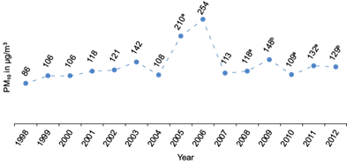
Fig. 1 Annual historical averages of PM10 in Mexicali. Data provided by the Secretaría de Protección al Ambiente (SPA) of the Government of the State of Baja California. a According to the SPA, the value can be sub-estimated due to the fact that the indicator was obtained with information of less than 75 % of the valid data. b Values estimated by the authors with data from the manual stations provided by the SPA. (Source: Pers. comm ).
Figure 2 shows the annual averages of PM10 occurred during the period from 2000 to 2012 and those projected until 2020 for Mexicali.
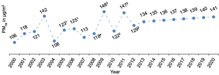
Fig. 2 Annual historical and projected PM10 averages for Mexicali. Data provided by the Secretaría de Protección al Ambiente (SPA) of the Government of the State of Baja California until the year 2012. From year 2013 are projections. For the purpose of such projections, the original values for 2005 and 2006 (i.e. values 210a and 254 of Fig. 1) were eliminated since they were extreme severe data and replaced by values estimated by the authors using regression models. Five regression models (i.e. exponential, linear, logarithmic, polynomial and power) were tested and was used that with the highest R2. a According to the SPA of the State Government, the value can be underestimated due to the fact that the indicator was obtained using information that was less than 75 % of the valid data.1 Data estimated by the authors using regression models. 2 Data estimated by the authors using data from the manual stations (COBACH, CONALEP, ITM, PROGRESO and CESPM) provided by the SPA. (Source: pers. comm .).
As shown in figure 2, PM10 in Mexicali has been showing a systematic increase year by year. If it remains so, it could reach average levels of around 141 µg/m3 of air (95 % IC: 134, 148) in the year 2020 according to the projected trend.
Scenarios
The following are the three scenarios established in the decrease of PM10 pollution levels for Mexicali:
(a) A total decrease per year starting from 2013 and until 2020.
(b) A reduction to the levels indicated by the NOM-025-SSA1-1993 (SSA 1993) of 50 mg/m3 from 2013 to 2020.
(c) A systematic reduction of about 8 % each year from 2013 to reach in 2020 comparable levels to those indicated by the NOM- 025- SSA1-1993 of 50 µg/m3.
Avoided cases
In this present study, avoided cases of mortality and morbidity are calculated combining local ERF with others that are likewise obtained from scientific publications, but the condition being that these should had been previously applied to communities in Mexico.
The number of avoided cases due to changes in pollutant concentration is estimated using the equation (1) (USEPA 2003, 2012), with the assumption that the effects of the pollutant on health are continuous, from the lowest to the highest levels. In other words, the assumption is that there are no threshold effects in the ERF.
H ij = R iC j N β ij (1)
In which:
H ij = Number of cases of impact on health i related to the concentration of the pollutant j.
Ri = Basal rate of mortality or morbidity for population N by effect i (cases / inhabitants / year).
C j = Change of the pollutant concentration j.
N = Exposed population (number of people).
β ij = Exposure-response function by effect i due to the exposure to the pollutant j (increase of cases / unit of concentration).
Percentage changes and variability
To visualize variability both in the number of avoided cases as in associated costs for each scenario proposed, their respective low, medium and high values are estimated. These follow similar criteria to that were applied in one of the studies conducted by the INECC (McKinley et al. 2003), because aside from having been done in the country, it addresses aspects that are very similar to those covered in the local study in as much as calculation of the effects of PM10 on the avoided cases of mortality and morbidity.
Mortality
To calculate the low, central and high values the aforementioned INECC study (McKinley et al. 2003) proposes using three ERF that indicate the percentage changes per each 10 μg/m3 of air, which are: 0.5 % for the low value used by Samet et al. (2000), 0.7 % for the central value used by Levy et al. (2000), and 1.4 % for the high value proposed by Evans et al. (2000). For this study, a 0.35 % percentage change is used to calculate the low level. This was taken from a time-series study performed with local data from Mexicali that can be found in scientific publications in Reyna et al. (2012). The 0.5 % from Samet et al. (2000) is used to calculate the central value, and the 0.7 % from Levy et al. (2000) is used to calculate the high value.
Emergency room visits due to asthma
No ERF estimated with local data was found to calculate the avoided cases of morbidity, thus the authors generated them using data from the region. The estimation of local ERF follows a procedure that is similar to that established in the scientific literature (Yang et al. 2009), which is based on auto-regressive semi-parametric models using as a measuring unit weekly counts of the cases, instead of daily counts. This method is well suited as to the limitations of local morbidity data, which represent total counts per week and not total daily counts. The time-series used are from 2005 to 2007. The method used in the estimation of local ERF, implements auto-regressive generalized additive models (GAM) of the Poisson family, where it is first found a baseline model in which the dependent variable are weekly counts of asthma emergency room visits, and as confounding variables are the trend, seasonality, temperature, relative humidity, holidays, vacation days and lagged values of the dependent variable depending on the case of the lag or lags where statistically significant values occur in residual autocorrelation coefficients. The trend, seasonality, temperature and relative humidity are smoothed with cubic spline functions, whereas holidays and vacations are introduced into the model as dummy variables. The degrees of freedom of each spline and the adequacy of the baseline model are determined once the coefficients of the partial autocorrelation of the residuals do not exceed confidence limits (α = 0.05). Afterwards, the pollutant and its lags are added to the baseline model one by one. The statistical significance of the associated regression coefficients is measured and the one showing more significance is selected. This coefficient is used to estimate the exposure-response function of the impact that the PM10 pollutant has on asthma.
The low, central and high levels of emergency room visits for asthma are calculated using weighed averages (WHO 1996): the percentage change mentioned by the INECC (McKinley et al. 2003) of 4 % (95 % CI: 1 %, 7 %) proposed by Schwartz et al. (1993) and the percentage change estimated locally in Mexicali of 2.5 % (95 % CI: 0.43 %, 4.7 %). Each percentage change and their confidence intervals (CI) are weighted with the inverse of their respective variances. Then the average is calculated to obtain the weighted percentage change for every 10 μg/m3 of PM10: 3.05 % (95 % CI: 0.64 %, 5.5 %). And thus, the low level is estimated with the left average confidence interval, the central level with averaged percentage change, and the high level with the right average confidence interval.
Hospitalizations due to asthma
The 2.5 % (95 % CI: 0.43 %, 4.7 %), local percentage change utilized for the asthma hospitalization is the same as that calculated for asthma emergency room visits since it is assumed that the number of hospitalizations in this location depends on the number of emergency room visits for this pathology, which in Mexicali represents 17 % (see "Health Data" section). On the other hand, the INECC study (McKinley et al. 2003) utilizes a 3.02 % (95 % CI: 2.05 %, 4.00 %) percentage increase, stating such is proposed by the World Bank.
For the purpose of the current study these two percentage increments are weighted in the same way that those to emergency room visits as explained above to obtain the average. This new 2.94 % (95 % CI: 1.79 %, 4.12 %) percentage increment is used to calculate the low, central and high levels of hospitalization due to asthma.
Restricted activity days (RAD)
Since no local dose-response functions were found to calculate the low, central and high levels of RAD; the decision was made to follow criteria established by WHO (1996). This proposes a percentage increment of 3.0 % (95 % CI: 2.1 %, 4.7 %) per 10 μg/m3 of air of PM10 which is an adaptation of the original percentage increment associate to the effects of PM2.5. The adaptation is made using the relation  . For our study the percentage increment is adapted to the relation
  that was calculated with the actual PM10 and PM2.5 levels in Mexicali. Therefore, the resulting incremental percentage utilized is 3.5 % (95 % CI: 2.4 %, 5.5 %) per 10 μg/m3 of PM10.
Mortality
In this study, the economic assessment of PHB for mortality is estimated by the human capital approach, with the present value of future income that an individual would perceive if he had not died prematurely, by using the following equation (Sanchez et al. 1998, USEPA 2012):
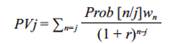 (2)
(2)
Where: PVj is the present value of future income for an individual of age j , Prob [n / j] is the probability that an individual of age j is alive at age n , w n is the average annual labor income by individual of age n , and r is the discount rate for the years after death.
In our study, the survival probabilities (i.e. n p x = 1- n q x ) were constructed using the new official mortality charts (i.e. n q x ) (AMA 1999), under the assumption that these probabilities have not changed with time since they were constructed.
The average annual labor income w n is obtained from the general average wages and not from the minimum wage, since it is based on the fact that most of the employed population of Baja California perceives income equal to or above the general average wage. General average wages for Baja California recorded by the Mexican Institute of Social Security (IMSS for its acronym in Spanish of Instituto Mexicano del Seguro Social) in 2011 reached 245.84 mexican pesos per day, this represents 4.11 minimum wage in the geographical area A of the country (source: National Commission on Minimum Wages CONASEMI for its acronym in Spanish of Comisión Nacional de los Salarios Mínimos, and INEGI). So the minimum wage is multiplied by this factor to calculate the general average wage corresponding to each year, assuming that the proportion of the number of minimum wages relative to average wages is maintained approximately the same year by year. Then, the average wages are converted to the corresponding US$ parity of each year, according to the historical series obtained from the Bank of Mexico. The minimum wages and parity of the dollar for the years 2013 to 2020 are projected following the tendency of previous years to 2013.
It is assumed that the employed population in Mexicali perceives average wages with a similar percentage distribution of that assigned by INEGI in the perception of minimum wages. This scenario means that different proportions of the employed population receive different wages. With the intention to balance this situation, a weighted average wage is estimated in function of the respective employed populations. It is assumed that the employed population that earns general average daily wages keeps a similar distribution to the employed population that earns minimum wages. Then the estimated weighted average daily wages of each year (US $85 in the period of the projected years) are multiplied by 313 officially working days per year in Mexico.
When calculating the present values of future income (PV ) for the loss of productivity due to premature death, a discount rate r of 3 % (see ecn 2) is applied to be consistent with other studies reported in the literature (Houtven and Cropper 1996, Sánchez et al. 1998).
Future income calculated by lost productivity are multiplied by the number of avoided death cases respective to every year, to finally obtain the costs attributable to avoided death cases for reducing the levels of PM10, under the proposed scenarios.
Morbidity
To calculate the assessment of morbidity effects (i.e. asthma hospitalizations, emergencies and restricted activity days), in this study, we used the costs associated to disease (i.e. direct cost of treatments and lost salaries due to days not worked), although there are other expenses: preventive or defensive expenses, (i.e. people living in a contaminated area are taking defensive measures to reduce the risk of sickness), also known as health production functions; and the contingent assessment, which is complicated and also expensive because of the implications of the number of gathered information and application of surveys.
As an indirect expense, restricted activity days are assessed, produced by the lost work days, for consequence of sickness, or for taking care of a sick person, or decrease of performance (Ostro 1987).
Costs associated to cases of emergency room visits due to asthma
For the purposes of this study, the associated costs to visits to the emergency room due to asthma are assessed based on the generated cost of the consultation, plus emergency attention, plus the expense of one work day lost. The produced expense of the medical consultation (i.e. US $157.3) is obtained from a study developed in the northeast of the country, by the University Hospital of the Regional Center of Allergy and Immunology of Nuevo Leon (Gallardo et al. 2007). The emergency attention expense is calculated with the estimated average (i.e. US $164.06) in the northeast study (i.e. US $97.33), with the estimated in a study made by the National Institute of Respiratory Diseases (INER for its acronym in Spanish of Instituto Nacional de Enfermedades Respiratorias) (Tapia and Casas 2009) (i.e. US $230.79). The values of consultation and attention from 2013 to 2020, are estimated based on prices obtained from the years 2006 and 2008, therefore a 3.20 % for the average inflation occurring in the 2008-2012 period was added to values from 2013 to 2020. It is assumed that the average inflation will remain without much variation until 2020. The cost of one lost business day is calculated from the average estimated salary. To obtain expenses attributable to the avoided cases by the decrease of PM10 levels, in the contemplated scenarios, the associated costs are multiplied by the avoided emergency cases.
Costs associated to cases related to hospitalization due to asthma
Hospitalization associated expenses are evaluated in this study with the costs generated by a day in bed rest (bed-day), inhalotherapy and the lost work days during the hospital stay. The average cost in Mexico of one bed-day in the hospital due to respiratory diseases in 2009 was US $340.78, inhalotherapy was US $3.33 (LaSalud 2009), while in the study made by the INER (Tapia and Casas 2009) there is an average expense of bed-day of US $333.75 (value obtained with 2007 prices). In the current study, we decided to use the US $340.78 value for bed-day and $3.33 for inhalotherapy. The values of bed-day and inhalotherapy used for the studied period from 2013 to 2020, are estimated based on prices obtained from 2009, therefore it is added a 3.20 % average inflation occurring in the 2008-2012 period. It is assumed that the average inflation will remain without much variation until 2020.
The average days of hospital stay due to asthma in Mexicali, are estimated to be 4 disability days (source: General Hospital Pers. comm .). The IMSS is forced to pay for the subsidy disabilities of 60 % of the last contribution salary, starting from the fourth day in disability. (See article 96 of the general law of IMSS and article 42 section II of the Federal Labor Law). This means, that the employee will lose 100 % of the first three days of disability, leaving only 40 % of the remaining days. Thus, corresponding hospitalization expenses are calculated by: cost of bed-day + inhalotherapy expense + cost of: the first three days of hospitalization stay x work day cost + one remaining day of hospitalization stay x 40 % of one work day. Then the avoided hospitalization cases are multiplied by the projected hospitalization expenses to obtain costs attributable to the avoided cases for reducing the PM10 levels in the contemplated scenarios.
Costs associated to restricted activity days
To calculate the restricted activity days (RAD), the procedure established by Ostro (1994) was used, where it is established that 20 % of RAD pertains to the number of lost work days and the complement (80 % of RAD) is assessed as the third part of the salary. In this manner, the total expense due to daily RAD is calculated with the sum of the 20 % plus a third of the 80 % of the RAD that is a net 46 % of daily productivity. It is assumed that the annual average number of net RAD per employed person in Mexicali is 18.99 (see section "restricted activity days"). Then, the net avoided RAD are multiplied by the total generated cost per daily restricted activity according to the pertaining year; to obtain the costs attributable to avoided RAD for reducing PM10 levels, under one of the established scenarios.
RESULTS
The 98th percentiles of the 24 hour averages of PM10 levels in Mexicali have historically marked an increasing trend every year, just like the annual averages. In fact, we can see in figure 2, that since year 2000, Mexicali has not been able to comply with the NOM-025-SSA1-1993 (SSA 1993) for the annual PM10 averages.
The social costs of the PHB estimated in each of the proposed scenarios are brought to present value using a discount rate of 3 % and presented as a percentage of state GDP reported in 2011.
Table I shows the local ERF used in this research along with the affected population and incidence rates. The ERF are shown as percentage increments as increases in the number of units of respective pollutant.
TABLE I Percentage changes per 10 mg/m3 of PM10 and their low, central and high levels, respectively
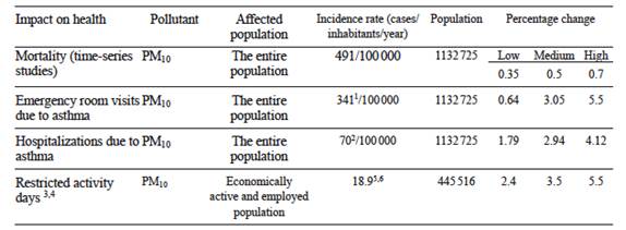
1Net incidence rate calculated after subtracting hospitalizations from emergency room visits.
2Incidence rate estimated using Imperial County, California, USA, data (see section "Hospitalization due to Asthma").
3The days of Hospital stay and emergency room visits both from the economically active and employed population are also taken as restricted activity days, and are thus subtracted from the total of restricted activity days.
4The coefficient taken from literature (WHO 1996) was obtained by using the employed population of 18 to 65 year olds. For the present study the economically active and employed population is assumed to be in the 15 to 64 year old age range.
5Net rate calculated after subtracting the days of hospital stay and emergency room visits of employed population from the total of the restricted activity days of the employed population.
6Obtained by adapting PM2.5/ PM10of Mexicali = 0.72.
Table II shows the low, central and high values of health and economic benefits estimated for each contemplated scenario in the study by effects of the reduction of PM10 in Mexicali. It shows the average avoided cases as well as the accumulated avoided cases for each health impact (2013-2020) with their corresponding expenses in US$ indicated in parentheses. The last line of the chart shows the expenses of each case (i.e. average and accumulated) as a state GDP percentage. The costs are brought to present value with a discount rate of 3 %. The GDP is the one reported in 2011 by INEGI (2012). For example, if PM10 pollution levels in Mexicali followed the projected trend over the studied years, but actions were carried out so that the average concentrations of each year succeed in being on the level of 50 μg/m3 marking the NOM- 025- SSA1-1993 (i.e. scenario b), the city would have a social benefit that would represent the central value of 3.56 % (low value: 2.50 %, high value: 5.37 %) of the state GDP reported in 2011. But, if these actions were about getting reductions of 8 % in the annual concentrations (i.e. scenario c), to reach in 2020 the level established by the norm; then the social benefit would represent a 2.13 % (1.50 %, 3.22 %) of the GDP. If the decision were about not conducting any action to decrease the levels of PM10, then the social expense would represent 5.59 % (3.92 %, 8.43 %) of the GDP.
Table II Social benefits for reducing PM10 levels under the established scenarios for Mexicali, in the projected period of years (2013─2020).
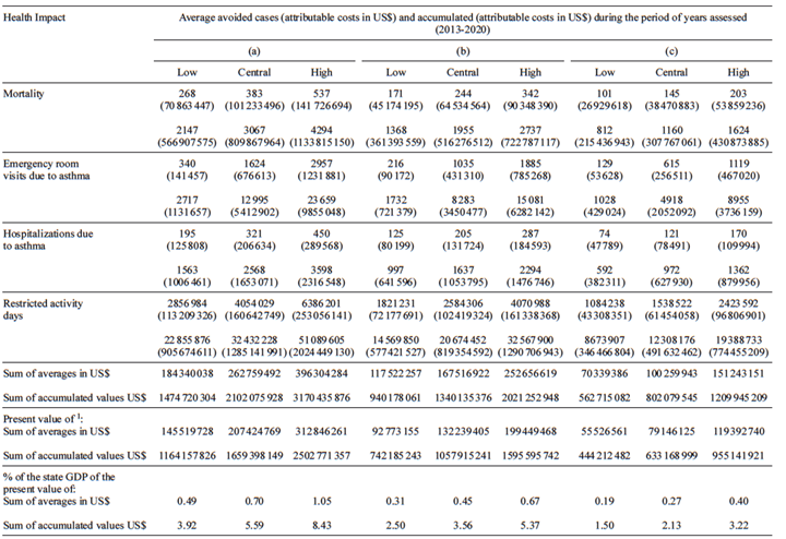
Scenarios: (a) a total reduction per year starting from 2013 and until 2020. (b) a reduction to achieve every year the levels indicated by the NOM-025-SSA1-1993 of 50 µg/m3, starting from 2013 and until 2020. (c) a reduction of a ~8 % every year starting from 2013 to achieve in 2020 approximate levels as those indicated by the NOM-025-SSA1-1993 of 50 µg/m3.
1Discount rate of 3 %.
GDP: Gross domestic product.
DISCUSSION
We would recommend identifying the specific type of control measures that could be implemented in order to reduce PM10 levels in Mexicali. Perhaps separating by sectors where there should be more actions taken to reduce pollution accordingly to the type of source and pollutant (i.e. stationary sources, area, mobile). In the 2005 Mexicali emissions inventory (ERG 2009), the area sources are the ones contributing the most PM10 and PM2.5, whereas the CO is predominant in mobile sources in roads. There is a "ProAire Mexicali 2011-2020" where there was more than 40 actions proposed aiming to reduce air pollution. It would be advisable to assess the economic benefit that would result from the implementation of each of the proposed actions, in order to prioritize those showing the greatest social benefit impact resulting from the decrease of PM10. The results of the current project in a first approach shed light about the social benefits and costs that would generate, for carrying out or not those actions on achieving reductions in pollutant PM10 according to the 2020 projected scenarios.
If nothing were to be done to reduce PM10 in Mexicali and let it follow the trend projected to 2020, there would be a social cost of around $1659 million dollars. If the decision is to take actions to reduce PM10 levels by about 8 % annually, future projections of 2020 show that the social cost would be reduced to about $1026 million dollars. However, if the decision was to direct actions to reducing PM10 each year to have annual average levels established by the NOM-025-SSA1-1993, then the projections indicate that the social cost would decrease to about $601 million dollars. Then, some obligatory questions to answer would be: What kind of ProAire actions would be the most profitable to make, in terms of social benefit to be achieved according to the proposed scenarios? That is, once the economic benefits that can be obtained depending on the desired scenario are known, the most profitable ProAire actions would be those efficiently impacting the reduction of PM10 and/or other pollutants such as CO; the latter as long as the implementation cost does not exceed the estimated economic benefit in the contemplated scenarios.
The results of this study could be underestimated, because the assessment was made using available data from the location, therefore, many aspects such as: the effects of long term exposure to the pollutants, or the inclusion of more diseases, or the use of the approximation "willingness to pay" instead of the approximation "human capital", were not considered. Neither was considered the financial burden generated from the costs of medication used to control asthma, since it varies because it depends on the quality control of the disease; for example, an asthmatic patient, receiving appropriate care, has an average expense of $635 dollars, whereas the cost for a patient not receiving adequate care may add up to $10 582 dollars (SSA 2000). Another important aspect to mention is that the economic benefits in the current study were assessed under scenarios that consider PM10 levels established in NOM-025-SSA1-1993. However, this standard was replaced with NOM-025-SSA1-2014 on August 20, 2014 (SSA 2014), implying that the public health benefits would rise even more as the permissible limit values for the concentration of PM10 became more strict. The reason why the NOM-025-SSA1-1993 was used rather than the current one, was because the latter was published by the Official Journal of the Federation after this study had been completed. Nevertheless, the results provided by this study as an initial assessment, would justify the implementation of air pollution control measures in Mexicali.
It is important to mention that there is a study (Torillo 2008) on the economic assessment of asthma in Mexicali due to the effect of reducing PM10 and O3, where the ERF are estimated through regression models known as error correction models. However, the methodology of these models apparently does not follow the conventional methodology with regards to ERF estimation that is widely used in Health Impact Assessment: there is not a previous baseline model controlling the confounding variables and lags. That is, two confounding variables are included in the model simultaneously (temperature and relative humidity) as well as two pollution variables PM10 and O3, not considering other important control variables such as days of the week, holidays, vacation days, analyzed years, trends, seasonality, among others. The metrics for these variables in the models are not consistent: 8-h mobile averages are used for the O3 variable while mobile averages are used for PM10 and daily averages are used for the other independent variables. The models used are linear, even when the dependent variable is discrete and with a very probable distribution function that is not normal. For the current study it was decided to maintain a conservative scenario, which is the reason why the ERF reported in the theses were not used. Nevertheless, the results from this study would come to reinforce the importance of the implementation of control measures that would aid to decrease the levels of air pollution in Mexicali.
CONCLUSSIONS
The study evaluates the benefits to health and the social cost for the reduction of the PM10 pollutant in Mexicali, under the three scenarios already described.
Scenario A supposes total reduction of PM10 to level zero, meaning the absence of this pollutant in a way that it is presented as the baseline to determine the cost for doing nothing to reduce the concentrations. Scenario B proposes to reach and keep every year, starting 2013, PM10 concentrations at the levels indicated in the NOM-025-SSA1-1993. Both scenarios only establish a frame of reference for the study but its real viability was not evaluated.
However, it would be feasible to reach a yearly reduction of 8 %, established by scenario C, (although its viability was not evaluated) by means of the conjunction of the actions established in the ProAire Mexicali 2011-2020. For that it is recommended to elaborate a cost-benefit study of the actions that ProAire establishes, determining the ones with the biggest effectiveness and profitability.
However, the effective role of the three levels of government summed to the intergovernmental management and the social co-responsibility, are a requisite to strengthen the public policies that allow the PM10 to reach the levels established in the referred norm.
Another important component is the high awareness of the main actors and decision makers; after years of bearing social struggles, health impacts, political costs and loss of economic competitiveness due to the bad air quality of Mexicali, the conditions are given to establish action of reduction of emissions suggested by scenario C.
It is recommended the establishment of an intergovernmental organ that involves business sector, academia and civil society; that could be in charge of establishing and to impulse the diary that eventually allows implementing and evaluating the actions of Pro-Air of Mexicali.

