Ground level chemical analysis of air transported from the 1998 Mexican–Central American fires to the Southwestern USA

 

Análisis químico a nivel de suelo del aire transportado desde los incendios de 1998 de México y América Central al suroeste de los EUA

 

Ignacio VILLANUEVA–FIERRO¹, Carl J. POPP², Roy W. DIXON³, Randal S. MARTIN⁴, Jeffrey S. GAFFNEY⁵, Nancy A. MARLEY⁶ and Joyce M. HARRIS⁷

 

¹ Departmento de Ciencias Ambientales, Becario COFAA, CIIDIR–IPN Unidad Durango, Sigma S/N Fracc. 20 de Noviembre II, Durango, Dgo., 34000. Correo electrónico: ifierro62@yahoo.com.

² Department of Chemistry, New Mexico Tech, 801 Leroy Place, Socorro, NM 87801.

³ Department of Chemistry, California State University at Sacramento, 6000 J Street, Sacramento, CA 95819.

⁴ Department of Civil and Environmental Engineering, Utah State University, 4100 Old Main Hill, Logan, UT, 84322.

⁵ Department of Chemistry, University of Arkansas at Little Rock, Little Rock, AR, 72204.

⁶ Graduate Institute of Technology, University of Arkansas at Little Rock, Little Rock, AR 72204.

⁷ Office of Oceanic and Atmospheric Research, ERL/CMDL, NOAA, 325 Broadway, Boulder, CO 80303.

 

Recibido octubre 2007
Aceptado agosto 2008

 

ABSTRACT

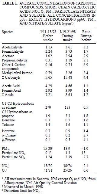
In May 1998, a large number of forest fires in the region of southern México and Central America, released huge amounts of contaminants that were transported over the Pacific Ocean, then, due to a change in air current direction, the primary contaminants and their secondary pollutant products impacted central New Mexico after 5 to 6 days transport time. The total distance traveled was approximately 3000 km from the fire source. Background measurements of a number of key chemical markers were taken before and during the haze incursion at a site located at Socorro, NM. A number of days before the haze episode in NM, large areas of Texas, Louisiana and the lower Mississippi River valley were also inundated by smoke from the fires. The sum of carbonyl compounds was 5.6 ppbv before and 15.5 ppbv during the smoke event; the sum of carboxylic acids went from 7.2 ppbv to 8.6 ppbv; C1–C2 hydrocarbons went from 270 ppbv to 133 ppbv; particulate NO₃– went from 0.1 to 1.3 µg/m³; SO₄^–2 went from 1.2 to 3.4 µg/m³; and PM₁₀ concentrations remained between the range measured before the episode (15–20 µg/m³). The results indicate the significant impact on a rural site from long range transport of primary and secondary smoke pollutants from biomass burning events and the importance of these species being primarily in the gaseous and fine aerosol size range. These fine aerosols are important as climate forcing agents and in reducing air quality and visibility.

Key words: biomass, fires, air quality, transport, stratosphere.

 

RESUMEN

En mayo de 1998, varios incendios forestales en la región sur de México y en América Central, emitieron enormes cantidades de contaminantes que fueron transportados al Océano Pacífico; entonces, debido a los cambios de dirección de las corrientes de aire, los contaminantes primarios emitidos, o como contaminantes secundarios, empezaron a llegar al centro de Nuevo México, después de 5 a 6 días del episodio. La distancia total del transporte fue de aproximadamente 3000 km desde la fuente de los incendios. Las mediciones de varios marcadores químicos fueron tomadas antes y durante la incursión del humo en Socorro, NM. Días antes de que llegara la contaminación a NM, grandes áreas de Texas, Louisiana y la parte baja del valle del Río Mississippi fueron cubiertas por el humo de los incendios. La suma de compuestos carbonílicos varió, antes del humo de 5.6 ppbv, a 15.5 ppbv durante la incursión del humo; la suma de ácidos carboxílicos varió de 7.2 ppbv a 8.6 ppbv; los hidrocarburos con 1 y 2 carbonos de 270 ppbv a 133 ppbv; los NO₃– en partículas de 0.1 a 1.3 µg/m³; los SO₄^–2 variaron de 1.2 a 3.4 µg/m³; las PM₁₀ se mantuvieron en el intervalo de antes de la incursión (15–20 µg/m³). Los resultados indican un impacto significativo en un sitio rural del transporte de larga distancia de contaminantes de humo primarios y secundarios provenientes de eventos de quema de biomasa y la importancia de estas especies se debe principalmente al intervalo de tamaño gaseoso y de aerosol fino. Estos aerosoles finos son importantes como agentes coadyuvantes al cambio climático y afectan la calidad del aire y visibilidad.

Palabras clave: biomasa, fuegos, calidad del aire, transporte, estratosfera.

 

INTRODUCTION

Atmospheric effects from large biomass fires (greater than a few thousand hectares) have received a great deal of interest in recent years, both in terms of effects on atmospheric chemistry (Crutzen and Andreae 1990, Crutzen and Carmichael 1993, Levine et al. 1995, McKenzie et al. 1995, Galanter et al. 2000, Marion et al. 2001, Thompson et al. 2001) and concern related to health effects when smoke impacts population centers (Lipari et al. 1984, Lewis et al. 1988, Nichol 1998). A number of studies of biomass fires have concentrated on fires occurring in the Amazon Basin (Andreae et al. 1988, Lee et al. 1998, Liu et al. 2000, Yamasoe et al. 2000, da Rocha et al. 2005, Schroeder et al. 2007) and savanna fires in Africa (Lee et al. 1998, Marion et al. 2000). There have also been a number of reports on large fires in other regions reported on fires in Southeast Asia (Brauer and Hisham–Hashim 1998, Nichol 1998, Weiss–Penzias et al. 2007) and the wildfires occurring in southern México and Central America in 1998 that resulted in decreased visibility and high aerosol concentrations in the United States at distances of 2500–4000 km from the fires. In southern México alone, the fires in 1998 were estimated to number >10,000 and consume more than 4000 km². More recently, in the year 2000 summer fire season in the United States, more than 80,000 wildfires in the western USA burned about 27,500 km² (Pelley 2000) raising issues of air quality effects in the western US due to these fire events. In addition to producing aerosols (Crutzen and Andreae 1990, Brauer and Hisham–Hashim 1995, Liu et al. 2000, Yamasoe et al. 2000), biomass fires have the potential to produce large quantities of oxygenated organic species such as aldehydes, ketones and carboxylic acids (Lipari et al. 1984, Andreae et al. 1988, McKenzie et al. 1995, Dibb et al. 1996, Lee et al. 1998, Yokelson et al. 1999, Holtzinger et al. 1999) as well as hydrocarbons (Larsen et al. 1992, Bernd et al. 2003), sulfate and nitrate (Andreae et al. 1988, Gorzelska et al. 1994, Dibb et al. 1996, Maenhaut et al. 1996), and associated gaseous pollutant species such as O3, NOx, and CO (Liu et al. 1999, Galanter et al. 2000, Marion et al. 2001, Thompson et al. 2001, Weiss–Penzias et al. 2007). Polycyclic aromatic hydrocarbons are also produced by biomass burning and found in the stratosphere (Jenkins et al. 1996, Amador–Muñoz et al. 2001, Mandalakis et al. 2005). Many of the literature reports dealing with products of biomass burning have been related to fireplace and wood burning stove emissions (Dasch 1982, Lipari et al. 1984, Zak et al. 1984, Andreae et al. 1988, Popp et al. 1996), to laboratory burns (McKenzie et al. 1995, Yokelson et al. 1996, Yokelson et al. 1997, Goode et al. 1999, Holtzinger et al. 1999) and to plume measurements using aircraft (Andreae et al. 1988, Gorzelska et al. 1994, Worden et al. 1997, Lee et al. 1998, Yokelson et al. 1999, Marion et al. 2000). Few measurements have been made on local or long range ground level effects from large forest/biomass fires (Dibb et al. 1996, Yamasoe et al. 2000, Liu et al. 2000), partly due to the difficulty of approaching hot, large fires and partly due to difficulties in a priori determination of a site that will be affected by the smoke plume. Large fires can contribute to atmospheric reactivity because long–range transport affords long reaction times for photochemical reactions and surface reactions on aerosol particles produced by the fires before wet and dry deposition occurs. In this study, organic and inorganic chemical species in the gaseous and aerosol phases were collected at ground level and have been identified and quantified under non–smoky and smoky conditions in May 1998 in central New Mexico. It is believed that the entire region was impacted by haze carried approximately 3000 km from the source of the spring 1998 Mexican/Central American fires. It should be noted that the background data collected before the haze incursion was part of a different study and when the regional haze developed, measurements were again taken at the same site used for the background data. For a number of days before the haze episode in NM, large areas of Texas, Louisiana and the lower Mississippi River valley were inundated by smoke from the fires. However, the haze in those places came from the same source but from a trajectory that went to the north of the fire and then to the west. Haze arriving into El Paso, Socorro and Albuquerque came from the trajectory shown in figure 1. The webpage http://www.cimms.ou.edu/ARM/smoke.html describes the meteorology for each day of May 1998.

 

EXPERIMENTAL

Field site and sampling protocol

The field sample site for the collection of carbonyl compounds, carboxylic acids and hydrocarbons is located in a rural, agricultural area in the Rio Grande flood plain near Socorro, NM (Lat. 34º, Long. 106º 7', pop.~9,500) in south–central New Mexico. The sample site had been used for several years for studies of biogenic emissions from cottonwood trees and for ambient sampling of atmospheric species in a rural, high desert environment. A week before the herein described fire event there was no visible evidence of haze attributed to the Mexican/Central American fires; ambient concentrations of carbonyl compounds, low molecular weight carboxylic acids and hydrocarbons were determined on a diurnal basis for two days (May 11–13, 1998) and aerosol samples were being collected for a different study. Neither of these studies were specifically in operation for smoke impact evaluation, but serendipitously allowed smoke plume impact to be evaluated at the site. A week later, the visibility in the region stretching from Albuquerque, NM (125 km north of Socorro) to El Paso, Texas (320 km south of Socorro) from the haze attributed to the fires was extremely poor and we again undertook a two–day sampling exercise (May 19–21, 1998) for the same species. Samples of carbonyl compounds and carboxylic acids were collected over 2–hour sampling periods with mid–sample times at 0800, 1200, 1600, 1800 and 2400 hr MDT. Hydrocarbons were collected over a 10–minute period at mid–sample times. NO_x and O₃ data were provided as one–hour averages by the city of Albuquerque, NM Air Quality Control Division Laboratory and El Paso, Texas. While these are urban sites and atmospheric species are affected by strong, local sources, the data do show some perturbation that may be attributed to the smoke. Unfortunately, no NOx or O3 instrumentation was available in Socorro at the time, and Albuquerque and El Paso were experiencing a haze episode at the same time underscoring the widespread, regional nature of the episode. Aerosol samples were collected on Teflon filters on the campus of New Mexico Tech in Socorro over periods of four days before and 1–3 days during the haze episode as described below. PM₁₀ samples were collected in Socorro using standard PM₁₀ sampling methodology.

Evidence for the source of the haze

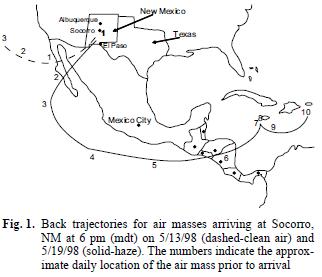
In addition to the obvious visual manifestation of increased haziness and significantly decreased visibility, satellite data support the changes occurring from the clean air period to the haze episode. Satellite images provided from the Louisiana State University Earth Scan Laboratory (Huh 1998) and the NASA TOMS System show the absence of smoke/haze during the clean air sampling period and the subsequent smoke/haze intrusion into Central New Mexico beginning about May 16 (sampling occurred May 19–21 during the most intense haze). While it is recognized that satellite imagery does not necessarily always reflect ground level concentrations, the regional and ground level visibility were severely degraded, a fact that was reflected in numerous headlines in the regional newspapers. Also, as a verification of the regional impact of the Mexican and Central American fires, an isentropic air trajectory model was used to examine the back trajectories of the air masses arriving to the Socorro, NM area during the study periods. Details on the methodology and uncertainties of the model can be found in Harris and Kahl (1994). Figure 1 shows modeled trajectories for the pre–smoke, clean period and for the smoke–influenced period clearly showing the long path of the air mass from México/Central America to New Mexico and, hence, the considerable time for products of the fires to be formed from secondary reactions.

Analyses

Gas phase aldehydes and ketones were sampled with Sep–Pac C₁₈ cartridges (Waters/Millipore Corp.) coated in the laboratory with acidified 2,4–dinitrophenylhydrazine (DNPH) following procedures previously described (Tanner et al. 1988, Zhou and Mopper 1990, Grosjean 1991) with specific descriptions regarding blanks, duplicates, detection limits, instrumentation, and calibration described in Gaffney et al. (1997). Briefly, the cartridges were cleaned with acetonitrile, coated with DNPH, wrapped in aluminum foil and stored in a refrigerator in dark containers. Air samples were pulled through a 5 µm Teflon filter and then through the cartridges at about 1 L/min, with air flow controlled by rotameters calibrated several times daily with mass flow meters (Aalborg Corp.). The samples were analyzed by HPLC (Waters Corp.).

Organic acid samples were collected from the gas phase at 2–hour intervals, corresponding to the collection schedule for the carbonyl compounds. Water mist nebulizers (40 mL capacity) specially constructed for trapping acids were used with the procedures described by Cofer et al. (1985) and modified by Popp et al. (1993). Specific descriptions of all protocols for blanks, duplicates, detection limits, instrumentation and calibration used are given by Gaffney et al. (1997). In general, ambient airflow of 6–8 L/min was pre–filtered (5 µm Teflon) and passed through the nebulizer. Following sample collection, the nebulizer was rinsed several times with distilled deionized water into volumetric flasks. The samples were treated with three drops of chloroform to prevent microbial decomposition, stored under refrigeration in dark glass bottles with Teflon–lined lids and analyzed by ion chromatography (Dionex Corp. 2000Si).

Gas analyses for NO_x and O₃ were performed in Albuquerque and El Paso by the city of Albuquerque Air Quality Control Division and by the El Paso City/County Health District according to EPA approved standard methods. Data were obtained from Albuquerque Air Quality Division personnel. All results were averaged to one–hour periods and are reported to the nearest 1 ppb.

Hydrocarbon samples were collected from the gas phase into 3.8 L Tedlar bags via a peristaltic pump and analyzed using GC/FID. Detailed methodology concerning calibration and quality assurance followed that of Martin et al. (1999). In short, 500–700 mL from each sample was cryogenically pre–concentrated prior to injection onto the chromatographic column (J & W Scientific; DB–1). The GC oven was temperature controlled, starting at –20 °C for three minutes, and then increasing at 5 °C per minute to a final temperature of 150 °C. Compound identifications were achieved by peak retention time comparisons with a qualitative standard and quantified by FID response comparison with an external, commercial standard. C1 and C2 compounds were not reported separately because the GC was set up to analyze isoprene and monoterpenes during the clean air period and there was insufficient time to recalibrate when the haze episode occurred.

Aerosol samples were collected, extracted, and analyzed using the procedures similar to those described by Dixon and Aasen (1999). Briefly, aerosol samples were collected on 47 mm, 1.0 µm Teflon filters (Cole–Parmer) in filter holders mounted upside down using flow rates of 40 mL min–1 set by flow through a critical orifice and checked with a rotameter. The low flow rates were used to integrate samples over several days and were not originally intended for the haze samples, but the same procedure was used for all sample sets for consistency. The filters were extracted with 0.5 mL of ethanol to "wet" the filter and deionized water or a preserving solution containing phosphoric acid (for analysis of S (IV) species not reported here) to a total volume of 20 mL. Sample extracts were analyzed for NO₃^1– and SO₄^2– using ion chromatography (Dionex 2000Si). Blank filters were extracted using the identical procedures to determine detection limits.

 

RESULTS AND DISCUSSION

Carbonyl compounds

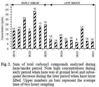
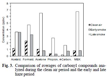
Average concentrations of carbonyl compounds are summarized in table I and shown in figures 2 and 3. The smoke episode occurred in two distinct stages during the three sampling days about a week after clear air measurements were made. During the early smoke stage (seven samples), the haze was evident at ground level and in the later stage (nine samples) the haze layer had lifted to a height of about 1–1.5 km above the ground at the sample site (from observation of nearby mountain peaks of known height) and the data in figure 2 compare these two periods. During the early haze period, the total carbonyls measured were 4.4 times higher than the previous week's clear air measurements. Overall, the total carbonyls were 2.7 times higher during the entire smoke episode than during the clean air period. The species exhibiting the greatest increases during the early smoke period compared to the clean air period were acetone (6.2 times), propionaldehyde (8.1 times), methyl ethyl ketone (MEK) (8.1 times) and other 4–carbon species (6.9 times and comparisons of the sample periods are shown in Fig. 3 and Table I). Formaldehyde and acetaldehyde, which normally contribute the largest percentages to total carbonyl compounds measured in ambient air in this region (Gaffney et al. 1997, Martin et al. 1999) showed relatively smaller increases of 2.0 times and 3.2 times, respectively, when comparing the hazy period to the clean air period. This observation is likely due to the greater reactivity and higher photolysis rates of formaldehyde and acetaldehyde relative to acetone and MEK. For instance, the atmospheric lifetimes of acetone and MEK with respect to OH radical at a concentration of 5 x 10⁶ molecules/cm³ are 10 and 2.3 days, respectively, while formaldehyde and acetaldehyde have lifetimes of 6.2 h and 3.5 h, respectively (Finlayson–Pitts and Pitts 1986). Because of the length of time for the smoke to arrive (5–6 days, Fig. 1), many of the carbonyl compounds originally generated in the fires would have undergone chemical transformation by reaction with OH radical and O3 or by photolysis. These processes would take larger carbonyl compounds and degrade them to smaller ones (Finlayson–Pitts and Pitts, 1986) or form other oxidized products (i.e. aldehydes, carboxylic acids). Subsequently, the shorter chain carbonyl compounds would likely have been regenerated by oxidation of hydrocarbons produced by the fires.

Carboxylic acids

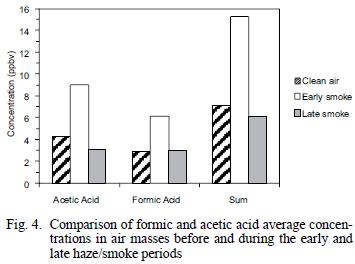
The average ambient concentrations of acetic and formic acids did not show increases similar to the carbonyl compounds. As shown in table I, only slight increases of 1.1 times (acetic acid) and 1.4 times (formic acid) were found when comparing overall averages for the clean air and hazy sample periods. However, when the clean air period is compared to the early (ground–level) smoke vs. the late smoke, increases similar to the aldehydes are evident (Fig. 4). As shown in figure 4 and table I, during the early part of the haze period, the acetic acid concentrations increased by a factor of 2.0 and formic acid increased by a factor of 2.1 over clean air values, similar to, but slightly lower than observed increases for the carbonyls compounds. While these carboxylic acid species have also been identified as major components in biomass burning (Lipari et al. 1984, Andreae et al. 1988, McKenzie et al. 1995, Dibb et al. 1996), it is likely that deposition, neutralization and scavenging by aerosols or rain may have attenuated the concentrations of these species during long–range transport, while oxidation to carboxylic acids was simultaneously taking place from hydrocarbons and carbonyl compounds produced directly and/or indirectly from the fires.

Hydrocarbons

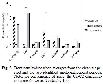
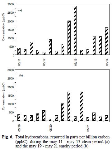
The mixing ratios for the C1–C2 and C3 (as propane) compounds are reported as such due to peak separation limitations imposed by operating conditions for the GC/FID system as discussed above. As can be seen in figure 5, the C1–C2 compounds were present in mixing ratios one to two orders of magnitudes greater than all of the other identified hydrocarbons, similar to comparisons for biomass combustion plumes reported elsewhere (Hao et al. 1998, Blake et al. 1998). In contrast to the previously discussed carbonyls and organic acids, examination of the hydrocarbon concentrations during the early and late smoky periods, in units of total parts per billion carbon (ppbC) shows that the higher values occurred during the latter period (see Fig. 6a). However, the change observed between the two smoky periods is similar to that observed over the duration of the clean air period (see Fig. 6b). C3s remained high during the early and late smoke periods. Toluene during the early smoke period was doubled, but during late smoke decreased by half, while isoprene, benzene, α–pinene and β–pinene were present above the values measured before the episode.

NO_x and O₃

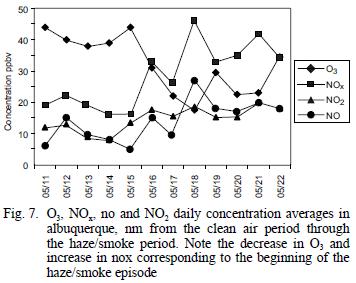
Average values for NO_x and O₃ concentrations measured in Albuquerque, NM and El Paso, TX during the clean air and hazy periods are summarized in table I and shown on a daily average basis in figure 7. Albuquerque is located 120 km north of Socorro, where all the other measurements were made, and El Paso is located ~300 km south. However, the haze was regional and was quite evident both in Albuquerque and El Paso, so even though the concentrations of NO_x and O₃ are expected to be higher at the urban sites than in rural Socorro, the relative changes should be valid for comparison. The NO_x concentrations in Albuquerque averaged 2.1 times higher and O₃ concentrations averaged 1.6 times lower during the smoke period when compared to the cleaner period. Similar comparisons for El Paso showed NOx to be 1.4 time higher and O₃ to be 1.2 times lower during the study period. As shown in figure 7, the daily average concentrations of both species were steady during the clear air period and began to change between May 15 and 16, about the time the haze became noticeable. For comparison, the average summer NO_x and O₃ concentrations found in Albuquerque during a previous study were 20 ppbv and 35 ppbv, respectively (Gaffney et al. 1997). Ozone concentrations might have been decreased by lower UV intensity during the smoke, while NOx concentrations could have increased due to meteorological conditions (inversion layer that also trapped smoke near the ground). Ozone concentration increases during biomass burning (Cooney 2008).

Particulate matter

In spite of the obvious haze present during the smoke episode when visibility was decreased significantly, PM₁₀ concentrations showed almost no difference in Socorro (Table I) or Albuquerque (Peyton 1998), and only an increase in PM₁₀ in El Paso on May 19–20. This is surprising because the haze obscured vistas of mountains 5–6 km distant when mountain ranges in the Socorro area are normally visible from 80–100 km. The particles causing the haze may have been too small to contribute significantly to the mass on the filters, but no particle size analysis was available at the time.

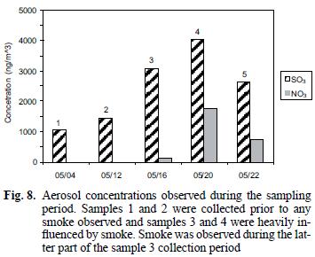
Soluble nitrate and sulfate associated with the particulate samples collected on the Teflon filters during the haze period were 13 and 2.7 times greater, respectively, than during the clear air period (see Table I and Fig. 8). It is likely that oxidation of SO₂ and NO_x produced during the fires is the source of the excess nitrate and sulfate associated with the particulate material. The increases for nitrate (Andreae et al. 1988, Gorzelska et al. 1994, Dibb et al. 1996) and sulfate (Andreae et al. 1988, Gorzelska et al. 1994, Dibb et al. 1996, Maenhaut et al. 1996) are consistent with previous observations. Gorzelska et al. (1994) reported enrichments of 8 times for SO₄^2– and 4 times for NO₃^1– in the boundary layer in smoke plumes.

 

CONCLUSIONS

This study suggests that ground level detection of a number of chemical species and precursors from smoke from biomass fires in southern Mexico such as aldehydes, ketones, short–chain carboxylic acids, and particulate–associated sulfate and nitrate was possible at great distances (approximately 3000 km) from the fires. Analysis of air associated with very unusual, regionally observed hazy conditions detected increases over clean air background levels. Some of these compounds would likely have undergone reactions during transport of the air mass, but study of such changes was beyond the scope of this study. In addition, concentrations of other species such as NO_x and O₃ may be affected. It is not evident from this study that ground level O₃ concentrations are enhanced long distances from large fires, even though strong evidence exists for the presence of high levels of fine aerosols and gaseous ozone precursors. This may be consistent with the strong optical absorption of the smokes that leads to the reduction of UVB which in turn drives the photochemical processes of ozone formation (Gaffney et al. 2002). In this study, no significant increases of PM10 levels were observed under very hazy conditions suggesting transport of only very small particles. These fine particles are important as climate forcing agents due to their optically high absorption and are also important as they may have significant health impacts. Hydrocarbon analyses yielded inconsistent results in that some increased (C3, benzene, isoprene, α–pinene, β–pinene) while some decreased (C1, C2). The results from this work clearly indicate that regional scale impacts from biomass burning must be considered when addressing air quality impacts from air toxics and fine aerosols.

 

ACKNOWLEDGMENTS

The authors acknowledge Dr. Oscar Huh, LSU Earth Scan Laboratory for access to satellite photos. We thank Dr. Waldemere Bejnar for sample site access and utilities and Ed Peyton and Matt Hind of the Albuquerque Air Quality Control Division for O3 and NOx data. We also thank Jennifer Knowlton for help with the hydrocarbon analyses.

 

REFERENCES

Amador–Muñoz O., Delgado–Rodríguez A., Villalobos–Pietrini R., Munive–Colin Zenaida, Ortiz–Marttelo R., Díaz–Gonzalez G., Bravo–Cabrera J.L., Gómez–Arroyo S. (2001). Partículas suspendidas, hidrocarburos aromáticos policíclicos y mutagenicidad en el suroeste de la Ciudad de México. Rev. Int. Contam. Ambient. 17, 193–204.        [ Links ]

Andreae M.O., Browell E.V., Garstang M., Gregory G.L., Harriss R.C., Hill G.F, Jacob D.J., Pereira M.C., Sachse G.W., Setzer A.W., Silva P.L., Talbot R.W., Torres A.L. and Wofsy S.C. (1988). Biomass–burning emissions and associated haze layers over Amazonia. J. Geophys. Res. 93, 11509–11527.        [ Links ]

Bernd R., Simoneit T., Rushdi A.I., Bin ABAS M.R. and Didyk B. M. (2003). Alkyl amides and nitriles as novel tracers for biomass burning. Environ. Sci. Technol. 37, 16–21.        [ Links ]

Blake N.J., Blake D.R., Sive T.Y., Rowland R.S., Collins J.E., Sachse G.W. and Anderson B.E. (1998). Biomass burning emissions and vertical distribution of atmospheric methyl halides and other reduced carbon gases in the South Atlantic region. J. Geophys. Res. D19, 101, 24151–24164.        [ Links ]

Brauer M. and Hisham–Hashim J. (1998). Fires in Indonesia: crisis and reaction. Environ. Sci. Technol. 32, 404A–407A.        [ Links ]

Cofer III W.R., Collins V.G. and Talbot R.W. (1985). Improved aqueous scrubber for collection of soluble atmospheric trace gases. Environ. Sci. Technol. 19, 557–560.        [ Links ]

Cooney C.M. (2008). Can a change in fire burning season affect air pollution?. Environ. Sci. Technol. 42, p 2713.        [ Links ]

Crutzen P.J. and Andreae M.O. (1990). Biomass burning in the tropics: impact on atmospheric chemistry and biogeochemistry. Science 250, 1669–1678.        [ Links ]

Crutzen P.J. and Carmichael G.R. (1993). Modeling the influence of fires on atmospheric chemistry. In: Fire in the Environment–The Ecological, Atmospheric and Climatic Importance of Vegetation Fires. (P.J. Crutzen, J.G. Goldammer, Eds.), Wiley, Chichester, pp. 89–105.        [ Links ]

da Rocha G.O., Allen A.G. and Cardoso A.A. (2005). Influence of agricultural biomass burning on aerosol size distribution and dry deposition in southeastern Brazil. Environ. Sci. Technol. 39, 5293–5301.        [ Links ]

Dasch J.M. (1982). Particulate and gaseous emissions form wood–burning fireplaces. Environ. Sci. Technol. 16, 639–645.        [ Links ]

Dibb J.E., Talbot R.W., Whitlow S.I., Shipham I.C., Winterle J., McConnell J., Bales R. (1996). Biomass burning signatures in the atmosphere and snow at Summit, Greenland: an event on 5, August, 1994. Atmos. Environ. 30, 553–561.        [ Links ]

Dixon R.W. and Aasen H. (1999). Measurement of hydroxymethanesulfonate in atmospheric aerosols. Atmos. Environ. 33, 2023–2029.        [ Links ]

Finlayson–Pitts B.J. and Pitts Jr. J.N. (1986). Atmospheric chemistry. Fundamentals and experimental methods, Wiley, NY. pp 496–510.        [ Links ]

Gaffney J.S., Marley N.A., Martin R.S., Dixon R.W., Reyes L.G., and Popp C.J. (1997). Potential air quality effects of using ethanol–gasoline fuel blends: a field study in Albuquerque, New Mexico. Environ. Sci. Technol. 31, 3053–3061.        [ Links ]

Gaffney J.S. Marley N.A., Drayton P.J., Doskey P.V., Kotamarthi V.R., Cunningham M.M., Baird J.C., Dintaman J. and Hart H.L. (2002). Field observations of regional and urban impacts on NO₂, ozone, UV–B, and nitrate radical production rates: nocturnal urban plumes and regional smoke effects. Atmos. Environ. 36, 825–833.        [ Links ]

Galanter M., Levy H. III and Carmichael G.R. (2000). Impacts of biomass burning on tropospheric CO, NOx, and O3. J. Geophys. Res. 105, 6633–6653.        [ Links ]

Goode J.G., Yokelson R.J., Susott R.A., Ward D.E. (1999). Trace gas emissions from laboratory fires measured by open–path Fourier transform infrared spectroscopy: fires in grass and surface soils. J. Geophys. Res. 104, 21,237–21,245.        [ Links ]

Gorzelska K., Talbot R.W., Klemm K., Lefer B., Klemm O., Gregory G.L., Anderson B., Barrie L.A. (1994). Chemical composition of the atmospheric aerosol in the troposphere over the Hudson Bay lowlands and Quebec–Labrador regions of Canada. J. Geophys. Res. 99, 1763–1780.        [ Links ]

Grosjean D. (1991). Ambient levels of formaldehyde, acetaldehyde, and formic acid in Southern California: Results of a one–year base–line study. Environ. Sci. Technol. 25, 710–715.        [ Links ]

Hao W.M., Ward D.E., Olbu G. and Backer S.P. (1994). Emissions of CO₂, CO and hydrocarbons from fires in diverse African savanna ecosystems. J. Geophys. Res. D19,101, 23577–23584.        [ Links ]

Harris J.M. and Kahl J.D.W. (1994). Analysis of 10–day isentropic flow paterns for Barrow, Alaska: 1985–1992. J. Geophys. Res., D12, 99, 25845–25855.        [ Links ]

Holzinger R., Warneke C., Hansel A. Jordan A., Lindinger W., Scharffe D.H., Schade G. and Crutzen P.J. (1999). Biomass burning as a source of formaldehyde, acetaldehyde, methanol, acetone, acetonitrile, and hydrogen cyanide. Geophys. Res. Lett. 26, 1161–1164.        [ Links ]

Huh O. (personal communication) (1998). Louisiana State University Earth Scan Laboratory, Baton Rouge, LA.        [ Links ]

Jenkins B.M., Jones A.D., Turn S.Q., Williams R.E. (1996). Emission factors for polycyclic aromatic hydrocarbons from biomass burning. Environ. Sci. Technol. 30, 2462–2469.        [ Links ]

Larsen F.S., McClennen W.H., Deng X., Silox G.D. and Allison K. (1992). Hydrocarbon and fromaldehyde emissions from the combustion of pulverized wood waste. Combust. Sci. Tech. 85, 259–269.        [ Links ]

Lee M., Heikes B.G. and Jacob D.J. (1998). Enhancements of hydroperoxides and formaldehyde in biomass burning impacted air and their effect on atmospheric oxidant cycles. J. Geophys. Res., 103, 13201–13212.        [ Links ]

Levine J.S., Cofer W.R. III, Cahoon D.R. and Winsted E.L. (1995). Biomass burning: a driver for global change. Environ. Sci. Technol. 29, 120A–125A.        [ Links ]

Lewis C.W., Baumgardner R.E. and Stevens R.K. (1988). Contribution of woodsmoke and motor vehicle emissions to ambient aerosol mutagenicity. Environ. Sci. Technol. 22, 968–971.        [ Links ]

Lipari F., Dasch J.M. and Scruggs W.F. (1984). Aldehyde emissions from wood–burning fireplaces. Environ. Sci. Technol. 18, 326–330.        [ Links ]

Liu H., Chang W.L., Oltmans S.J., Chan L.Y. and Harris J.M. (1999). On springtime high ozone events in the lower troposphere from Southeast Asian biomass burning. Atmos. Environ. 33, 2403–2410.        [ Links ]

Liu X., Van Espen P., Adams F., Cafmeyer J. and Maenhaut W. (2000). Biomass burning in southern Africa: individual particle characterization of atmospheric aerosols and savanna fire samples. J. Atmos. Chem. 36, 135–155.        [ Links ]

Lyons W.A., Nelson T.E., Williams E.R., Cramer J.A. and Turner T.R. (1998). Enhanced positive cloud–to–ground lightning in thunderstorms ingesting smoke from fires. Science 282, 77–80.        [ Links ]

Maenhaut W., Salma I., Cafmeyer J., Annegarn H.J. and Andreae M.O. (1996). Regional atmospheric aerosol composition and sources in the eastern Transvaal, South Africa, and impact of biomass burning. J. Geophys. Res. D19, 101, 23631–23650.        [ Links ]

Mandalakis M., Gustaffson Ö, Alsberg T., Egeback A.L., Reddy C.M., Xu L., Klanova J. Holubek I. and Stephanou E.G. (2005). Contribution of biomass burning to atmospheric polycyclic aromatic hydrocarbons at three European background sites. Environ. Sci. Technol. 39, 2976–2982.        [ Links ]

Marion T., Perros P.E., Losno R. and Steiner E. (2001). Ozone production efficiency in savanna and forested areas during the ESPRESSO experiment. J. Atmos. Chem. 38, 3–30.        [ Links ]

Martin R.S., Villanueva I., Zhang J. and Popp C.J. (1999). Nonmethane hydrocarbon, monocarboxylic acid, and low molecular weight aldehyde and ketone emissions from vegetation in central New Mexico. Environ. Sci. Technol. 33, 2186–2192.        [ Links ]

McKenzie L.M., Hao W.M., Richards G.N., Ward D.E. (1995). Measurement and modeling of air toxins from smoldering combustion of biomass. Environ. Sci. Technol. 29, 2045–2054.        [ Links ]

Nichol J. (1998). Smoke haze in Southeast Asia: A predictable recurrence. Atmos. Environ. 32, 2715–2716.        [ Links ]

Peyton E. (personal communication) (1998). Albuquerque air quality division, Albuquerque, N.M.        [ Links ]

Popp C.J., Zhang L. and Gaffney J.S. (1993). Organic carbonyl compounds in Albuquerque, NM air: a preliminary study of the effects of oxygenated fuel use. In: Alternative Fuels and the Environment; (F.S. Sterrett, Ed.) CRC Press, Boca Raton, FL, 61–74.        [ Links ]

Popp C.J., Martin R.S., Jones D., Knowlton J.A., Bonkemeyer P. and Galanis S. (1996). Environmental Division Abstracts, 13^th Rocky Mountain Regional A.C.S. Meeting, Denver, CO.        [ Links ]

Schroeder W., Csiszar I. and Morisette J. (2007) Quantifyig the impact of cloud obscuration on remote sensing of active fires in the Brazilean Amazon. Remote Sens. Environ. DO:10.1016/j.rse.2007.05.004.        [ Links ]

Tanner R.L., Miguel A.H., de Andrade J.R., Gaffney J.S. and Street G.E. (1988). Atmospheric chemistry of aldehydes: enhanced peroxyacetyl nitrate formation from ethanol–fueled vehicular emissions. Environ. Sci. Technol. 22, 1026–1034.        [ Links ]

Thompson A.M., Witte J.C, Hudson R.D., Guo H., Herman J.R. and Fujiwara M. (2001). Tropical tropospheric ozone and biomass burning. Science 291, 2128–2132.        [ Links ]

Worden H., Beer R. and Rimsland C.P. (1997). Airborne infrared spectroscopy of 1994 western wildfires. J. Geophys. Res. 102, 1287–1299.        [ Links ]

Yamasoe M.A., Artaxo P., Miguel A.H. and Allen A.G. (2000). Chemical composition of aerosol particles from direct emissions of vegetation fires in the Amazon Basin: water–soluble species and trace elements. Atmos. Environ. 34, 1641–1653.        [ Links ]

Yokelson R.J., Susott R., Ward D.E., Reardon J. and Griffith D.W.T. (1997). Emissions from smoldering combustion of biomass measured by open–path Fourier transform infrared spectroscopy. J. Geophys. Res. 102, 18865–18877.        [ Links ]

Yokelson R., Griffith D.W.T., Ward D.E. (1996). Open–path Fourier transform infrared studies of large–scale laboratory biomass fires. J. Geophys. Res. 101, 21067–21080.        [ Links ]

Yolkelson R.J., Goode J.G., Ward D.E., Susott R.A., Babitt R.E., Wade D.D., Bertschi I., Griffith D.W.T. and Hao W.M. (1999). Emissions of formaldehyde, acetic acid, methanol, and other trace gases from biomass fires in North Carolina measured by airborne Fourier transform infrared spectroscopy. J. Geophys. Res. 104, 30109–30125.        [ Links ]

Weiss–Penzias P., Jaffe D., Swartzendruber P., Hafner W., Chand D. and Prestbo E. (2007). Quantifying Asian and biomass burning sources of mercury using the Hg/CO ratio in pollution plumes observed at the Mount Bachelor observatory. Atmos. Environ. 41, 4366–4379.        [ Links ]

Zak B.D., Einfeld W., Church H.W., Gay G.T., Jensen A.L., Trijonis J., Evey M.D., Homann P.S. and Tipton C. (1984). The Albuquerque winter visibility study, Vol. I: Overview and data analysis, Sandia Report SAND84–173/1, Sandia National Laboratories, Albuquerque, NM. pp 1–67.        [ Links ]

Zhou X. and Mopper K. (1990). Measurement of sub–parts–per billion levels of carboxyl compounds in marine air by a simple cartridge tarpping procedure followed by liquid chromatography. Environ. Sci. Technol. 24, 1482–1485.        [ Links ]