


 nueva página del texto (beta)
 Inglés (pdf)
 Artículo en XML
 Referencias del artículo
 Enviar artículo por email
 Citado por SciELO
  Similares en
SciELO
Similares en
SciELO 
 Permalink
INTRODUCTION
Calculating physical characteristics of water bodies such as volume, surface area, and shape is a challenging process because of the complex underwater topography. The water body’s floor is usually irregular, with elevations and depressions that do not follow a specific pattern and therefore are difficult to model with mathematical equations. The height of the water level (H), volume (V), surface area (A), and the shape of the surface area are parameters that are not linearly interrelated. Determining these parameters, using a known value from the previously mentioned parameters (H, V, or A), will allow erosion modelers, hydrologists, geohydrologists, and ecologists. Currently, geographic information system (GIS) is able to deploy programming languages to develop tools that respond to complex problems. This approach generates information about the storage capacity in a dynamic way to support management policies dealing with flood risk zones and minimum water levels for maintaining ecologically healthy areas and other water resource issues.
Several methodologies exist to calculate morphometric parameters, such as height, volume, area, maximum depth, and the average depth of water bodies. The first studies that relate volumearea-depth used the ratio between average depth and maximum depth in addition to sinusoidal parameters (such as lake bottom profile) to do so (Lehman, 1975; Neumann, 1959). Sima and Tajrishy (2013) presented a model that relates volume-area-elevation using data from remote sensors and analytical procedures such as a power model and a truncated pyramid model. This approach results in highly parameterized equations that relate morphometric values. Moreno-Amich and Garcia-Berthou (1989) used echo sounding to relate morphometric characteristics of depth-area measurements for developing hypsographic curves and generating a bathymetric map.
Johansson et al. (2007) proposed two new mathematical models that interrelate morphometric values: the volume development, which is an equation based on the A-V relationship curve (Vd) and the hypsographic development parameter, which is the integration of A-depth and V-depth relation curves (Hd). These models require three inputs: V, maximum depth, and A. Recent methodologies that use unmanned aerial vehicles measure the height of the terrain through LIDAR (Laser Imaging Detection and Ranging) and surface water vehicles that measure the depth (bathymetry) through high-resolution echo sounding. These data sources are processed in GIS and generate accurate DTMs (Erena et al., 2019). Regardless of the methodology, however, the equations that relate the morphometry variables inherit the uncertainty of the complexity and spatial variability of underwater topography (Rode et al., 2010). Chen et al. (2018) presented a method that uses 3D geometry of a dam with which the volume and floodplains are calculated. The algorithm uses precipitation and water stage values as input data. It then simulates the floods in two sections: the floodplain and the 3D model from which the morphological parameters are obtained. Despite being an efficient model, it is limited as to what input data it will accept. Thus, none of the methods shown above are capable of offering solutions where morphological values interact with each other to respond to the needs of hydrologists.
To address these uncertainties, this study develops a technique that fully estimates the H-V-A of water bodies using computational techniques through 3D models that include bathymetry and the surrounding terrain topography. This technique used the water column below the level of the water surface projected onto each pixel of the DTM; this calculation was applied to the entire study area to delineate the extension of the water body. The V or A was the reference variables deployed in an iterative algorithm until the error threshold was accomplished.
STUDY AREA
The Bustillos Lake is in the endorheic Cuauhtémoc Basin, and the lake has an area of 3,298.15 km2. A mountain range, called Sierra Azul, surrounds it in the north-northeast; on the western flank are Mennonite colonies where the terrain slope is below 1%. In addition, the town of Anahuac is in the south. The Bustillos Lake is between the quadrant coordinates 28° 38’ 51’’ N - 28° 28’ 27’’ N and 106° 57’ 3’’ W - 106° 38’ 50’’ W in the Cuauhtémoc municipality in the Mexican state of Chihuahua (Figure 1).
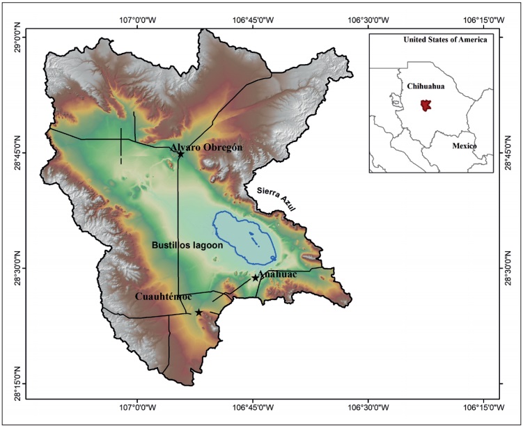
Source: self-made with data retrieved from INEGI (2019).
Figure 1 Study area where the algorithm was applied. The Bustillos Lake in Chihuahua.
Because the Cuauhtémoc Basin is between the semi-humid climate of the Sierra Madre Occidental and the Chihuahuan Desert, the region’s weather is warm and semi-dry (Kottek et al., 2006). The approximate elevation of the Cuauhtémoc region is 2,100 m above sea level (m.a.s.l), and the average annual temperature ranges from 6.9 to 21 °C, with an average annual rainfall of about 528 mm y-1 (Servicio Meteorológico Nacional, 2019).
MATERIAL AND METHODS
This methodology employed a personal computer with an Intel i3-8100 3.6 GHz processor, 48 GB RAM, and two SSD of 1 TB each. For this computational development in GIS, it is essential to have a DTM that includes the bathymetry of the study area for generating the hydrological characteristics of the water body: the 3D topobathymetric model of the Bustillos Lake (spatial resolution of 5 meters)(Rojas-Villalobos et al., 2018) (Figure 2).
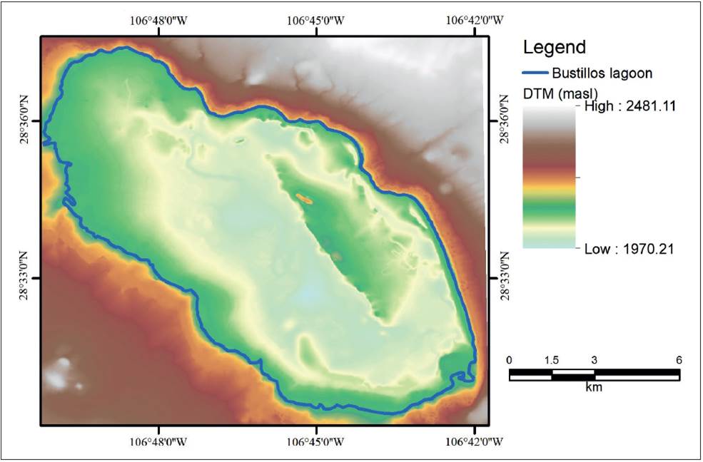
Source: self-made with data retrieved from Rojas-Villalobos et al. (2018).
Figure 2 DTM of the Bustillos Lake.
The software used for GIS processing was ArcMap® version 10.6 of Environmental Systems Research Institute, ESRI (ArcMap, 2019). The 3D process tool called Surface Volume, which requires the DTM and the height of the water level as input data, performed V and A calculations (numerical results), and Python® version 2.7.13 was the language to encode the algorithm (Python Language Reference, 2019).
The algorithm can capture one of the various input data, and as a result, it can generate the rest of the output data; for this reason, is cataloged as a single-input, multiple-output data algorithm. The algorithm uses one of the following input values: the height of the water level H, the storage V, or the A of the water body (Figure 3). All calculations are in the International System of Units.

Source: self-made.
Figure 3 The schematic diagram shows single-inputsand multiple-output data for the iterative algorithm.
The algorithm was designed using the following criteria. The algorithm is divided into two sections and depends on the input data: i) H water height in meters above sea level (m.a.s.l); ii) V (m3) or A (m2). Some of the process used in the second section refers to procedures in the first section.
The Surface Volume tool calculates the water volume in the column between H and each pixel of the DTM, thus generating the V and A of the water body. These two results were used to obtain the maximum and average depth, and both were estimated with the following equations:
where AD is average depth (m), V is the volume (m3), A is the surface area of the water body (m2), MD is maximum depth (m), H is the height of water level (m), and Hmin is the height of the water body floor (m), which was extracted from the properties of the raster. The Map Algebra tool, included in ArcMap®, was used to perform the extraction of the raster that represents the water surface filtering of all pixels that were less than or equal to H. Then, a conversion tool saves the surface water raster as a polygon (vector data) in a shapefile format file or geodatabase.
When the second process starts, the user captures (or by default) an error threshold (ET)(%) required to stop the iteration process and the value of V or A used to compute output information. V or A assumes the value of reference (Ref) that is used to compare with the new iterated values (V or A). The threshold limit (TL) is the value that stops the iteration and is the product of V or A multiplied by ET. Three initial variables were as follows: Step equal to 1 used to increase or decrease H, H equal to 1 meter above the bottom of the lake, and direction (Dir) equal to “upward”. The iteration starts with the H and the Surface Volume tool that calculates new data (ND = V or A). If the absolute value of the difference between Ref and ND is less than TL, the algorithm proceeds to execute the procedures for calculating the output information such as raster image and polygon shape of the lake. Otherwise, H continues increasing and generating ND until the absolute difference between Ref and ND is less than TL (e.g., 50 m3 or 70 m2). If ND surpasses Ref, H decreases at the halfway point of the previous step (e.g., 0.5 m.) until the absolute difference between ND and Ref is less than TL. If the TL is not accomplished and the ND surpasses Ref, H starts to increase with a new step (e.g., 0.25 m.). This iteration stops when the absolute difference is less than TL, and the algorithm calculates output data. The algorithm diagram is shown in Figure 4.

RESULTS AND DISCUSSION
Table 1 shows the results of three simulations with different data input. For the second and third models, the data resulting from the first simulation was used as input data (V and A) for the crosscomparison since the V-A estimates are calculated directly from the height, and it is not necessary to iterate data.
Table 1 Results in the implementation of the algorithm in Python language. Study site: the Bustillos Lake, Chihuahua, Mexico. Error threshold = 0.01%. * Input data.
| Error Threshold Area km3 |
Height m.a.s.l |
Volume hm3 | Area km2 | Average depth m |
Maximum depth m |
Iterations | Processing times |
|---|---|---|---|---|---|---|---|
| 0.01 | 1973.7* | 289.1004 | 114.256 | 2.5302 | 3.4860 | 0 | 1.407 |
| 0.01 | 1973.69 | 289.100* | 114.255 | 2.5302 | 3.4859 | 17 | 13.668 |
| 0.01 | 1973.69 | 289.0111 | 114.252* | 2.5295 | 3.4852 | 14 | 11.466 |
Source: self-made.
The results of the cross-comparison of H-V-A showed that the differences are 0.003, 0.0034, and 0.000039%, respectively. These values are below the established error threshold of 0.01% and represent a height differential of less than one micrometer, which is negligible in the lake modeling scale. The DTM covers an area of 246.00 km2, which contains the entire lake and the surrounding area in a buffer greater than 1000 meters. The lake has a storage capacity of 360.52 hm3 and a surface area of 122.8 km2 before extending to the floodplains at 1974.3 m.a.s.l. The processing time depends directly on the number of pixels of the DTM used in the modeling and not on the lake area itself. Two DTMs were modeled with different pixel dimensions: DTMa) 5.879 (width) x 3.925 (height) corresponding to 576.8 km2 and DTMb) 3.198 (width) x 3.077 (height) equivalent to 246.00 km2. Each pixel maintains a spatial resolution of 5 meters. The iteration number varies between 16 and 22 because of fluctuations in the calculated volume, which does not exceed the reference volume in each of the iterations. These variations can decrease or increase the number of iterations and, consequently, the calculation time (Table 2). The dimension of the DTM is directly and linearly related to the processing time in each iteration. The DTMa model is 2.34 times larger than DTMb, and this ratio is repeated in the average runtime of 1.84 seconds per iteration for the DTMa and 0.78 seconds per iteration for DTMb. This advantage can be exploited by hydrological modelers that require real-time results because they do not have to consider the simulation area but rather the number of pixels contained in the DTM.
Table 2 Iterative model processing times with various storage volume input values using two DTMs with different pixel dimensions. Pixel spatial resolution: 5 meters.
| DTM Tested Area (km3) | Volume (m3) | Iterations | Processing time (s) | Seconds per iteration |
|---|---|---|---|---|
| 576.80 (DTMa) | 100 | 16 | 29.78 | 1.86 |
| 576.80 | 150 | 22 | 39.85 | 1.81 |
| 576.80 | 200 | 18 | 33.46 | 1.85 |
| 576.80 | 250 | 21 | 38.61 | 1.83 |
| 576.80 | 300 | 16 | 29.82 | 1.86 |
| 246.00 (DTMb) | 100 | 16 | 12.77 | 0.79 |
| 246.00 | 150 | 22 | 16.84 | 0.76 |
| 246.00 | 200 | 18 | 14.24 | 0.79 |
| 246.00 | 250 | 21 | 16.35 | 0.77 |
| 246.00 | 300 | 16 | 12.83 | 0.80 |
Source: self-made.
The advantage of the iterative model is that it uses three-dimensional models based on measurements such as bathymetry and topography that represent reality at a given spatial resolution. The accuracy of the algorithm results, as well as the raster and flood shape, depend on three factors: accurate data for constructing the DTM, the spatial resolution of the pixel, and the selected error threshold. The complexity of underwater morphometry is shown in Figure 5. Four layers of the water surface are superimposed at every 25 centimeters in height in a stack to distinguish the nonlinearity of morphometric characteristics geographically.

Sources: self-made with data from Rojas-Villalobos et al. (2018).
Figure 5 Water surface coverage map at different heights above sea level of the Bustillos Lake.
The value of morphometric variables as the height of the water surface rises above the DTM does not show a constant pattern that can define a precise correlation between them (Figure 6).
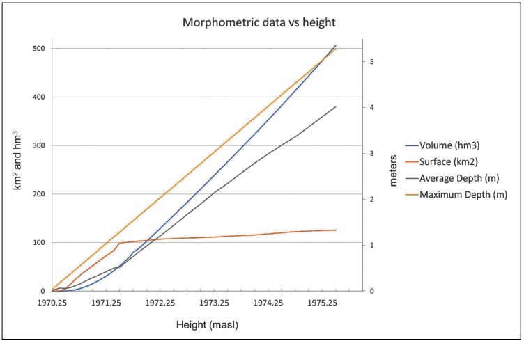
Source: self-made.
Figure 6 Comparative graph of volume, surface area, average depth, and maximum depth according to the height above sea level.
The increase in the water elevation and the surface growth is similar at constant rates until 1971.5 m.a.s.l. because the lake bottom is flat, and for each meter of elevation, the coverage of the lake water is significantly extended. The water body is shallow due to the relationship between the volume and the extension reached by the lake. From 100 km2, the raise of the surface continues being constant but at a slower rate. The volume rises slowly in the first meter of depth, and above this elevation, the volume tends to increment linearly at a higher rate. In this way, it is possible to establish equations by segments for each of the parameters but not a system of equations that integrates the five variables as determined by the algorithm.
RECOMMENDATIONS
The iterative algorithm proved efficient in finding every one of the morphometric values of the Bustillos Lake within the proposed error threshold. The following recommendations, however, are listed.
The purpose of this document is not to evaluate the quality of DTM. To obtain accurate morphometric data and detailed and realistic coverage maps, however, the DTM must meet geographic accuracy (lowest error) in all three axes (X, Y, and Z).
Use reasonable pixel dimensions of the study area. When there are more pixels, there is more process time.
This iterative model is not restricted to using a DTM; it is possible to replace it with a triangulated irregular network (TIN), which is composed of triangles where the vertices are elevation points.
The algorithm can be implemented in any programming language that handles spatial components, such as Python-GDAL®, R® statistics, or Magik Smallworld®.
Despite the PC computing capacity, the algorithm can be applied to any computer with minimum requirements: 4 GB RAM, HD with enough space to store the simulations (100-150 GB), and a fast processor (2.0 GHz +).

