


 nueva página del texto (beta)
 Inglés (pdf)
 Artículo en XML
 Referencias del artículo
 Enviar artículo por email
 Citado por SciELO
  Similares en
SciELO
Similares en
SciELO 
 Permalink
INTRODUCTION
What is the effect of violence on Mexico’s economy? Does violence negatively affect growth determinants such as labor productivity? The causes, effects, escalation, and spread of drug-related violence in Mexico have attracted much attention in recent years (Pan et al. 2012; Ashby and Ramos, 2013; Enamorado et al. 2014; Dell, 2015; Shrik and Wallman, 2015; Osorio, 2015; Torres-Preciado et al. 2015; Balmori de la Miyar, 2016; Cabral et al. 2016; and Bel and Holst, 2018). But while much recent literature has focused on the effects of drug-related crimes on aggregate economic activity, little attention has been paid to the growth determinants themselves, to the spatial spillover effects, and the spatial disparities that emerge from changes across space and time. These issues are the focus of this paper, in which we estimate a spatial panel regression for Mexico’s 32 states over a period of 14 years, 2003-2016, with the effects of violence on labor productivity of prime concern.
Spatial panel regression is characterized by its two-dimensionality, allowing data to interact across space and time (Elhorst, 2010 and Millo and Piras, 2012) and a combination of time series for each geographic or location unit that includes realistic assumptions concerning spatial heterogeneity at each point in time. Because estimation parameters are not homogenous or stationary throughout the data set but vary across space (Anselin et al. 2008) dependence among the observations can be addressed by including the spatial lag of the dependent variable, explanatory variables and/or the error term. Panel data add more variation and less collinearity among the variables, increasing both the availability of degrees of freedom and the efficiency of the regression estimates (Elhorst, 2010). Berry et al. (2007) suggest that global models that assume a common functional structure are not able to address spatial heterogeneity and, as a result, to correctly characterize a data-generating spatial process. Additionally, most of the literature on the effect of violent crime on growth ignores not only the presence of spatial autocorrelation in the dataset, but also the specification of additional endogenous explanatory variables and the spatial error process. To overcome these limitations, this study estimates a spatial panel regression model using the Generalized Method of Moments (GMM), which allows not only for spatial dependence in the dependent and exploratory variables at each point in time, but also in the error process correcting for the endogeneity of both the spatially lagged dependent variable and other potentially endogenous explanatory variables (Fingleton and Le Gallo, 2008; Bouayad-Agha and Védrine, 2010; Miao et al. 2015). GMM estimation is more flexible than Maximum Likelihood (ML) because it relaxes the normality assumption for the errors while still producing consistent estimators (Croissant and Milo, 2019).
MODEL SPECIFICATION
In its general form the spatial panel regression equation is given by:
where
We specify the terms in Eq. (1) as follows:
Table A1 in Appendix 1 includes the expected signs, sources, and a brief description of each variable. Eq. (2) controls for regional characteristics that explain changes in labor productivity. Briefly, the dependent variable represents labor productivity or GDP per employed worker in state i. Wages are average daily wages reported to the Mexican Social Security Institute (IMSS). DRV stands for drug-related violence including the combined total of extortion, gun homicide, and kidnapping per 100,000 inhabitants. K is public investment related to physical infrastructure and service provision. HumanCapital considers the share of the workforce with at least high school diploma. Following the analysis of Gallaway et al. (1967) and Rappaport (2005), AltUnemp intends to capture the effect of labor mobility by estimating the difference of unemployment rate in state i and the weighted average distance of unemployment rates in the rest of the country except state i≠j. Agglomeration identifies employment density by considering the number of employed people per km2. Border variable considers the geographic proximity to the United States by calculating the GDP weighted by the distance between state i and the nearest U.S. port of entry. Following Acs et al. (2002), Buesa et al. (2010), and Wang et al. (2016), Patents intends to capture the effects of innovation on GDP per worker by considering the number of patents per 100,000 inhabitants. ManuLQ tries to capture location effects by including the employment location quotient of the secondary sector. FinancialCrisis is a dummy variable that captures the effect of the financial crisis during the 2008-2009 period. In specifying the AltUnemp and Border variables we calculate distances using the great circle distance. In order to eliminate or reduce simultaneity between the right side of Eq. (2) and the dependent variable we use a one-period lagged explanatory variables. Table 1 shows the descriptive statistics and variance inflation factors (VIF).
Table 1: Descriptive Statistics and Multicollinearity Diagnostics
| Regression Variables | Mean | SD | Max | Min | VIF |
|---|---|---|---|---|---|
| Labor Productivity | 31,227 | 29,035 | 233,866 | 11,929 | - |
| Wages | 225.6 | 32.3 | 337.4 | 159.4 | 2.81 |
| Human Capital | 0.2981 | 0.0643 | 0.5228 | 0.1682 | 2.08 |
| Agglomeration | 135.35 | 517.30 | 3,127.45 | 2.84 | 2.15 |
| Patents Rate | 0.9810 | 1.5592 | 10.5889 | 0.0002 | 1.71 |
| Public Investment | 945.90 | 718.77 | 6,868.24 | 54.95 | 1.25 |
| Drug-Related Violence | 11.70 | 12.24 | 99.31 | 0.0005 | 1.48 |
| Alternative Unemployment | 6.51 | 346.71 | 1,062.204 | -1,214.15 | 1.42 |
| (ln) Border Distance | 17.68 | 1.31 | 22.43 | 15.60 | 2.59 |
| Manufacturing Location Quotient | 0.9673 | 0.2229 | 1.4464 | 0.1239 | 1.78 |
| Financial Crisis | 0.1538 | 0.3612 | 1.0 | 0.0 | 1.10 |
| Govt. Spending on Public Security | 7.09 | 3.45 | 22.9 | 1.74 | 2.12 |
| Marijuana Seizures | 51,593.1 | 105,581.3 | 692,695.8 | 0.0 | 1.78 |
| Cocaine Seizures | 3,562.9 | 31,086.76 | 543,478.6 | 0.0 | 1.10 |
| Guns Seizures | 494.2 | 1,072.46 | 11,248 | 0.0 | 1.21 |
Source: Authors’ estimations using R
Eq. (2) relies on the assumption of zero correlation between violent crime rates and the error term. However, Enamorado et al. (2014) and Osorio (2015) find empirical evidence suggesting that the escalation and diffusion of drug-related violence in Mexico were in part the result of increased law enforcement that in turn intensified violence and instability among criminal organizations. Enamorado et al. (2014) suggest that the capture of drug trafficking organizations leaders along with the military offensive might have contributed to instability within criminal groups. Osorio (2015) found that increased law enforcement (e.g., arrests, seizures of assets, seizures of drugs, and seizures of weapons) helps explain the intensification of violence between criminal organizations. Sharkey and Torrats-Espinosa (2017), on the other hand, use grants received by law enforcement agencies as an instrument variable to control for changes in violent crime rates (homicides, aggravated assaults, and robberies) when examining its impact on economic mobility across 1,355 U.S. counties. In the same vein, Werb et al. (2011) take into account a drug policy perspective and conduct a systematic review of scientific evidence to explore the effects of drug law enforcement (e.g., share of drug arrests of the total of all arrests, drug seizure arrests, and police expenditure) on drug market violence (e.g., violent crime and homicide rates, principally). Their review indicates that increasing law enforcement produces an escalation of gun violence and high homicide rates (Werb et al. 2011).
In examining the determinants of state labor productivity, failing to address the correlation between time-varying explanatory variables, for example drug-related violence, and omitted variables can produce biased estimators (Fingleton and Le Gallo, 2008; Sharkey and Torrats-Espinosa, 2017; Croissant and Millo, 2019). To test for the relationship between law enforcement and changes in drug-related violence, we estimated a Bivariate Moran’s I to track changes in this relationship across space and time. By generating 10,000 random permutations and using the queen contiguity criterion to represent the spatial structure of the data, Table 2 shows Bivariate Moran’s I results indicating that marijuana and guns seizures are positively associated with drug-related crimes in neighboring states. The relationship between drug-related violence and marijuana seizures goes from 0.38 in 2008 to 0.43 in 2011, including a significant escalation between 2010 and 2011, the peak period of Mexico’s drug war. Based on the Bivariate Moran’s I results, we therefore attempt to push the literature forward by considering a spatial GMM technique that allows for spatial dependence of both the dependent variable (ρ) and the error term (λ), with instrumental variables estimation (IV) to control for endogeneity of drug-related violence. The instrumental variables include government spending on public security, seizures of drugs (specifically marijuana and cocaine), and guns seizures. Similar to the explanatory variables, the instrument variables also include a one-period lag. Implementation is via the spgm command of the splm package in R. We thus go beyond the analysis of Decker et al. (2009), Pan et al. (2012), Cabral et al. (2016), Torres-Preciado et al. (2017), and Bel and Holst (2018) by using instrumental variables and by considering the spatial lags in labor productivity (ρ), drug-related crimes (θ), and the error term (λ).
Table 2: Bivariate Moran’s I between Law Enforcement (Marijuana, Cocaine, and Guns Seizures) and Drug-Related Violence from 2008 to 2015
| Year | Marijuana Seizures |
Cocaine Seizures |
Guns Seizures |
| 2008 | 0.3776 *** | 0.0404 | 0.1519 * |
| 2009 | 0.3863 *** | 0.0069 | 0.0926 |
| 2010 | 0.4825 *** | -0.0474 | 0.2139 ** |
| 2011 | 0.4282 *** | 0.0403 | 0.2467 ** |
| 2012 | 0.2642 *** | -0.0161 | 0.1261 * |
| 2013 | 0.1522 * | -0.0739 | 0.0174 |
| 2014 | 0.1309 * | 0.0891 | 0.0540 |
| 2015 | 0.1221 * | -0.0402 | 0.0300 |
Note: ***,**,* Statistically significant at 1%, 5%, and 10%. Bivariate Moran’s I is calculated in GeoDa using 10,000 random permutations and the queen contiguity matrix.
DATA ANALYSIS
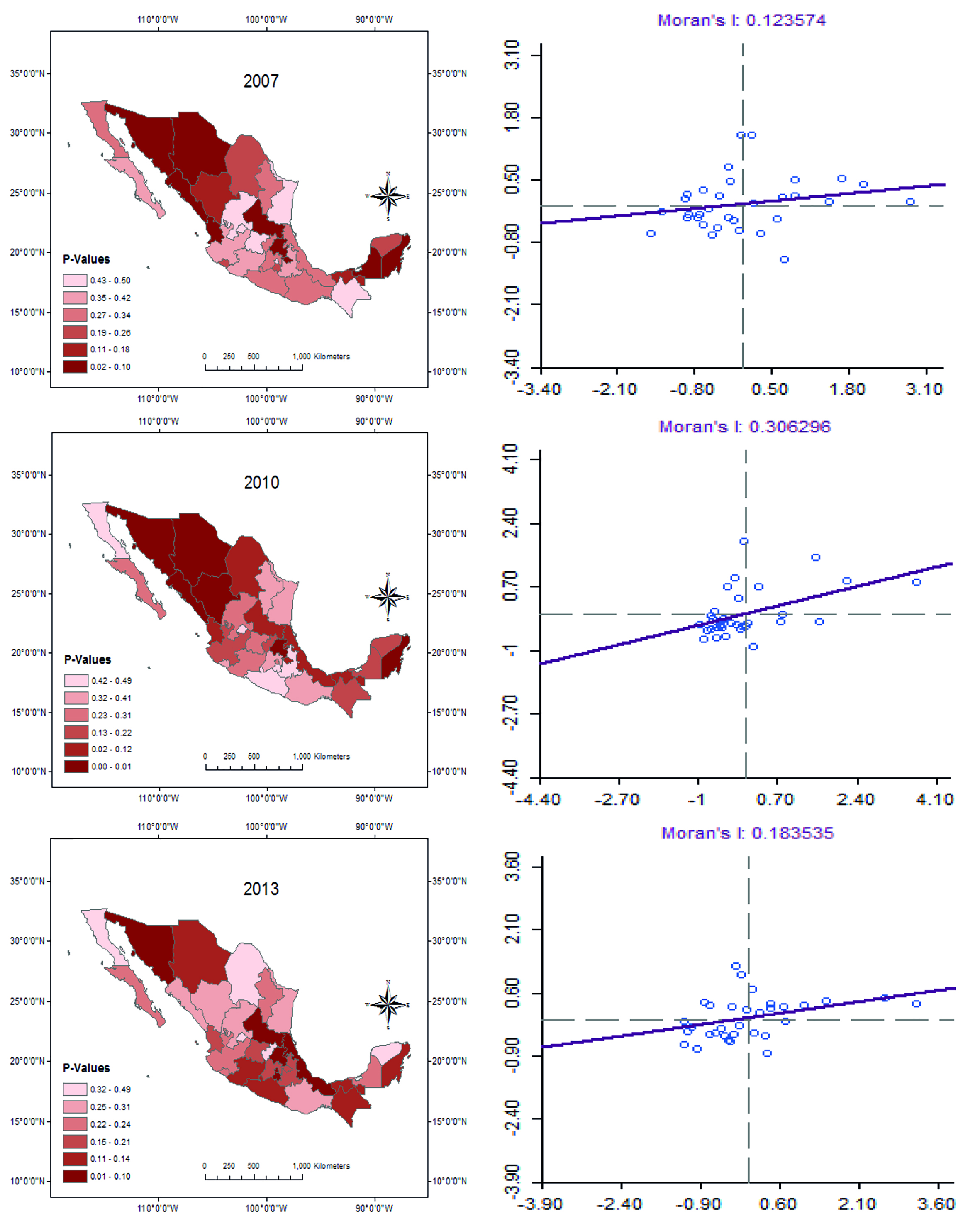
The key variables in this study are drug-related violence and labor productivity. A prior step was to consider whether they are spatially autocorrelated, “the tendency for nearby values on a map to be dependent” (Griffith and Arabia, 2010: p. 417). Two of the most widely used indices of spatial autocorrelation are Moran’s I and Geary’s C. Table 3 computes these statistics for Mexico’s states each year from 2003 to 2016. There clearly is spatial clustering. Global indicators of spatial autocorrelation are not, however, able to assess regional patterns of spatial autocorrelation. Local Indicators of Spatial Autocorrelation (LISA) are required. Figures 1 and 2 map the Local Moran’s I of drug-related violence and labor productivity and combine global and local indicators by displaying the quantile maps on the left and Moran scatterplots on the right. Figure 1 shows that despite the increase of drug-related violence after 2007, its spread across Mexican states was uneven: high violence rates initially clustered in northern border states, specifically the region known as Golden Triangle, which include the states of Chihuahua, Durango, and Sinaloa, in addition to the state of Sonora, but after 2010, it spread to non-border states, particularly states located across the Pacific zone (i.e., Baja California Sur, Guerrero, Michoacán, Morelos, Quintana Roo, and Veracruz). These results align with Enamorado et al. (2014) and Osorio (2015), who suggested that the strategy of Mexican government to combat organized crime after 2006 might have played a role in contributing to spread the violence across Mexican states.
Table 3: Global Indicators of Spatial Autocorrelation
| Drug-Related Violence | Labor Productivity | |||
|---|---|---|---|---|
| Year | Global Moran’s I | Geary’s C | Global Moran’s I | Geary’s C |
| 2003 | 0.1541* (0.0661) |
0.7456** (0.0421) |
0.0366 (0.1539) |
1.0608 (0.6817) |
| 2004 | 0.2282** (0.0225) |
0.6940** (0.0159) |
0.0388* (0.1003) |
1.0731 (0.7116) |
| 2005 | 0.2377** (0.0232) |
0.6838*** (0.009) |
0.0290 (0.1437) |
1.0804 (0.7168) |
| 2006 | 0.0935 (0.1428) |
0.77* (0.0567) |
0.0298 (0.1133) |
1.0828 (0.7167) |
| 2007 | 0.1236* (0.1001) |
0.8155* (0.0917) |
0.0300 (0.1132) |
1.0819 (0.7215) |
| 2008 | 0.1629* (0.0537) |
0.8125* (0.097) |
0.0414* (0.0877) |
1.0697 (0.7094) |
| 2009 | 0.2246** (0.0201) |
0.7525* (0.0505) |
0.0626* (0.0944) |
1.0292 (0.6262) |
| 2010 | 0.3063*** (0.008) |
0.6772* (0.0164) |
0.0621* (0.0929) |
1.0317 (0.6445) |
| 2011 | 0.2557** (0.0153) |
0.7117** (0.0252) |
0.0597* (0.0757) |
1.0424 (0.6649) |
| 2012 | 0.2036** (0.0382) |
0.7246** (0.0273) |
0.0798* (0.067) |
1.0138 (0.593) |
| 2013 | 0.1835** (0.0428) |
0.7534** (0.046) |
0.0645* (0.0915) |
1.0246 (0.6296) |
| 2014 | 0.1166 (0.1126) |
0.8202* (0.0997) |
0.0687* (0.0983) |
1.0122 (0.603) |
| 2015 | 0.1136 (0.1032) |
0.8174 (0.117) |
0.0814 (0.14) |
0.9265 (0.3335) |
| 2016 | 0.1371* (0.0758) |
0.6894** (0.0194) |
0.0635 (0.1804) |
0.9178 (0.2915) |
Note: ***,**,* Statistically significant at 1%, 5%, and 10%. Global Moran’s I and Geary’s C statistics are calculated in R using 10,000 random permutations and the queen contiguity criterion.
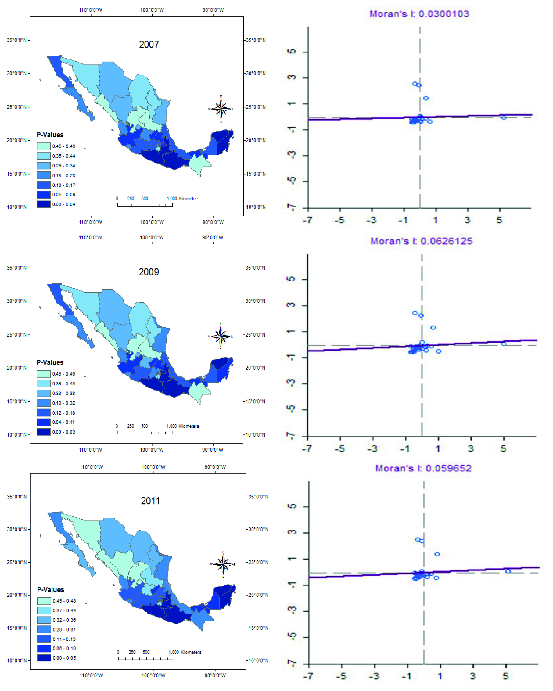
Source: Executive Secretary of the National System for Public Security (SESNSP). Maps and Moran’s scatterplots elaborated by the authors using ArcMap and GeoDa, respectively. LISA estimates use the queen criterion of contiguity. Inference is based on 10,000 random permutations.
Figure 1: Local Moran’s I of Drug-Related Violence (Homicide, Kidnapping, and Extortion) per 100,000 Population for Selected Years
Source: Institute of Statistic, Geography, and Information (INEGI). Maps and Moran’s scatterplots elaborated by the authors using ArcMap and GeoDa, respectively. LISA estimates use the queen criterion of contiguity. Inference is based on 10,000 random permutations.
Figure 2: Local Moran’s I of Labor Productivity for Selected Years
Over the same time span what happened to labor productivity? Figure 2 shows that labor productivity also clusters in geographic space. There was a weak but statistically significant presence of positive spatial autocorrelation in Hidalgo, Puebla, and Queretaro (center region), Jalisco (southwestern), and Yucatan, Quintana Roo, and Campeche (southeastern), respectively. Guerrero, Oaxaca, and Tabasco (south) in contrast, are characterized by the clustering of low-low labor productivity values. The Golden Triangle region (Chihuahua, Durango, and Sinaloa), on the northern region, also shows a spatial regime of similar labor productivity levels, but it is not statistically significant. According to Mexico’s Central Bank (Banxico), over the period 2007-2015, the states of Aguascalientes, Jalisco, Nayarit, Puebla, and Quintana Roo, showed the largest changes in labor productivity growth. Based on Banxico’s 2016 report, spatial clustering of high-high values in Figure 2 might be explained by the dynamism in the manufacturing sector.
Model Results
In estimating a first-order SARAR specification, we used the spatial GMM technique to allow for time-variant instrumental variable estimation (government spending in public security, seizures of drugs, and seizures of guns) to control for endogeneity in drug-related violence. We also considered different spatial weight matrices with both contiguity and distance criterions: both the queen and rook-based spatial weights (Wq and Wr) were used while inverse distance was used for the distance-based weight criterion (Wd1 and Wd2), with inverse weighted distance matrices based on the k=4 nearest neighbors and a specified distance of ≤ 600 km. We selected a distance threshold of ≤ 600 km because it is the average great circle distance from state i to Mexico City. Lastly, VIF calculation included both the explanatory variables and instrumental variables. Briefly, none of the VIF statistics are greater than 3 (see Table 1).
Table 4 shows the GMM spatial panel regression results. Briefly, average daily wages reported to Mexican social security are negative and highly statistically significant for all spatial weight matrices specifications. In our view, this result might be explained by a mismatch between an increasing labor force and stagnation in formal-sector occupation affecting productivity per worker. In a somewhat similar vein, Quinn and Rubb (2006: p. 148) examined the education-occupation matching on wages and productivity suggesting that “…in a country like Mexico we still find overeducated individuals because Mexico has a relative abundance of jobs that require low levels of education attainment” producing an adverse impact on wages and productivity. The spatial lag of GDP per worker (ρWY) shows statistically significant spillover effects indicating that growing productivity levels in neighboring states are positively related to productivity levels in a given state economy. Productivity levels appear to be explained by public investment rather than changes in wages. However, this result is not significant when considering the distance-based criterion Wd2. As expected, the distance from state i to the nearest U.S. port of entry plays a positive and statistically significant role in determining states’ GDP per worker, confirming the importance of location factors, especially for export-oriented industries (Jordaan, 2012). Mexico’s border states are strongly integrated to the business cycle of the U.S. economy particularly U.S. southern states (Phillips and Cañas, 2008).
The results also suggest the presence of agglomeration effects. Positive signs indicate a positive influence of labor pooling, low transaction costs, and agglomeration of economic activities on labor productivity levels. However, negative signs indicate that agglomeration costs such as high transaction costs and high crime rates overcome agglomeration benefits. Drug-related violence, the combined total of gun homicide, kidnapping, and extortion rate per 100,000 population, has a negative and statistically significant effect on GDP per employed worker except when considering the queen criterion Wq. Similarly, for all considered row-standardized spatial weight matrices, drug-related violence produces statistically significant negative spillover effects in a given state’s economy. Taking into account the increase and spread of drug-related crimes over the time period of the study, these results point out that drug-related crimes tend to cluster, exerting negative influences on the economy not only at the state level, but also across states.
Table 4: GMM Spatial Panel Regression Results using Fixed Effects Dependent Variable: GDP / Employed Worker
| Explanatory Variables | Wd1 | Wd2 | Wq | Wr |
|---|---|---|---|---|
| Wages i,t-1 | -0.6535*** (-3.31) |
-0.6400*** (-3.80) |
-0.7571*** (0.0179) |
-0.7305*** (-3.71) |
| Public Investment i,t-1 | 0.0645*** (3.30) |
0.0246 (1.43) |
0.0266* (1.71) |
0.0290* (1.85) |
| Human Capital i,t-1 | 0.0450 (1.09) |
0.0177 (0.46) |
0.0024 (0.06) |
0.0108 (0.26) |
| Alternative Unemployment i,t-1 | -0.00002 (-0.66) |
-0.00001 (-0.83) |
-0.00001 (-0.86) |
-0.00001 (-0.81) |
| Agglomeration i,t-1 | -0.4786*** (-5.72) |
-0.573*** (-7.49) |
-0.5471*** (-7.14) |
-0.5037*** (-6.44) |
| U.S. Border i,t-1 | 0.6965*** (13.88) |
0.7556*** (4.65) |
0.7692*** (16.89) |
0.7748*** (16.64) |
| Patents i,t-1 | 0.0021 (0.45) |
0.0023 (0.53) |
0.0021 (0.49) |
0.0017 (0.38) |
| Manufacturing Location Quotient i,t-1 | 0.0489 (0.82) |
0.0220 (0.41) |
0.0290 (0.53) |
0.0265 (0.48) |
| Drug-Related Violence i,t-1 | -0.0203** (-2.21) |
-0.0170** (-2.14) |
-0.0132 (-1.34) |
-0.0193* (-1.92) |
| W ∙ Drug-Related Violence i,t-1 | -0.0098** (-2.29) |
-0.0065** (-2.19) |
-0.0058* (-1.66) |
-0.0062* (-1.70) |
| Financial Crisis i,t | -0.0334** (-2.57) |
-0.0199 (-1.53) |
-0.0219* (-1.91) |
-0.0242** (-2.07) |
| ρ i,t | 0.4034*** (2.94) |
0.4423*** (3.39) |
0.4055** (2.42) |
0.3282** (2.15) |
| λ i,t | -0.0058 | 0.1207 | 0.0427 | 0.0678 |
| Hausman Test for Spatial Modelsϯ | 117.83 [0.00] |
125.76 [0.00] |
267.38 [0.00] |
120.43 [0.00] |
| Robust LM Test for
Spatial Lag DependenceϮ |
19.85 [0.00] |
20.66 [0.00] |
32.61 [0.00] |
32.64 [0.00] |
| Robust LM Test for
Spatial Error DependenceϮ |
20.74 [0.00] |
17.25 [0.00] |
36.03 [0.00] |
36.22 [0.00] |
| LM2 Test of no spatial autocorrelationϮ |
1.08 [0.28] |
0.35 [0.73] |
1.94
[0.06] |
1.96
[0.05] |
Note: *,**,*** Statistically significant at 10%, 5%, and 1%, respectively. t-statistics are in parenthesis. t-statistics are not available for the λ parameter. Wq and Wr stands for Queen and Rook contiguity criterion. Wd1 and Wd2 stands for inverse distance using k=4 and a distance threshold of ≤ 600 km. ϯChi-Square Test Statistic Value. ϮLagrange Multiplier Test Statistic Values (LM). p-values are in brackets.
Testing for robustness, the Hausman test for spatial panel data models in Table 4 led us to reject the null hypothesis that the preferred model is random effects: a fixed effects model is a better choice. Briefly, the Hausman test indicates that we can reject the assumption that individual-specific effects are not correlated with the explanatory variables. In the same vein, robust LM tests for the spatial lag of the dependent variable (ρ) and the spatial lag of the error term (λ) reject the null hypothesis of no spatial dependence in each, suggesting that the SARAR specification is correct. Regarding the latter, the inclusion of λ allows accounting for omitted exogenous spatially correlated effects on the dependent variable (Miao et al. 2016 and Kelejian and Piras, 2017). The LM2 test of no spatial autocorrelation in the residuals fails to reject the null hypothesis for the inverse distance spatial weight matrices (Wd1 and Wd2) but not for the queen and rook criteria (Wq and Wr), thus suggesting that the SARAR specification using the inverse distance criterion, specifically Wd1 and Wd2, is a better specification than using Wq and Wr.
SUMMARY AND CONCLUSIONS
There is a growing concern in the literature about the impact of drug-related crimes on the economy. However, most of the empirical literature has omitted the potential effect of spatial dependence and spatial heterogeneity. This study contributes to the literature by shedding more light on the impact of drug-related violence on Mexican states’ economy by analyzing the relationship between drug-related crimes and GDP per worker over the 2003-2016 period utilizing a spatial econometrics framework.
Our ESDA results indicate the presence of spatial patterns in the dataset, justifying the inclusion in our models of the spatial lag of both drug-related crimes and labor productivity. In terms of drug-related violence, global indicators of spatial association show a statistically significant increase of spatial clustering over time. Similarly, the Local Moran’s I of spatial association confirms the presence of local spatial patterns in GDP per worker employed and drug-related violence. Bivariate Moran’s I estimations indicate that law enforcement in a specific state, specifically marijuana and guns seizures, is associated with drug-related violence in neighboring states. These ESDA results validate the use of a first order spatial lag in the dependent variable and in drug-related violence. The spatial patterns of the relationship between illicit drugs enforcement and violent crimes rates confirms the necessity of using spatially lagged instrumental variables to address the endogeneity of drug-related violence, allowing testing for causality and reducing bias estimation.
Drug-related violence had a negative effect on labor productivity at the state level between 2003 and 2016, and also exerted negative spillover effects on regional economies. On the other hand, agglomeration produces a negative and statistically significant effect on GDP per worker, indicating that the presence of agglomerations costs such as high crime rates outweighs the positive effect of agglomeration economies. States’ GDP weighted by the distance to the nearest U.S. port of entry confirms positive and highly statistically significant impact of location factors on workers’ productivity.
In line with these findings and in keeping with the recent spatial econometrics literature (LeSage and Fischer, 2008; Hoang and Goujon, 2014; Kopczewska et al. 2015; Lim and Kim, 2015; and Ramajo et al. 2017), we confirm that spatial panel regression analysis points to the necessity of regional policy coordination among the states to reduce spillovers of drug-related violence and their negative effect on economic growth. Further research extensions should disaggregate labor productivity by economic sectors to assess the severity of each sector to the increase and spread of drug-related crimes across space and time. There is consensus in the literature that growth and development depend on the accumulation of human capital (Becker et al. 1994; Soares and Naritomi, 2007; and Justino, 2011). It is important to evaluate whether Mexico’s War on Drugs has been contributing to reductions in human capital accumulation by increasing internal or forced displacement of workers. In terms of modeling and estimation, further research extensions might consider a spatial dynamic panel data model to explore the short- and long-run dynamics between drug-related violence and labor productivity. Following Cárdenas and Rozo (2008), a growth decomposition exercise can contribute to test the hypothesis of a structural change in Mexico’s economy over the War on Drugs. Lastly, even though this study compares estimation results by considering different spatial weight matrices, particularly the contiguity and inverse distance criteria, according to LeSage (2014), a Bayesian perspective of spatial panel regression model comparison might well improve not only the model specification in terms of identifying the appropriate spatial weight matrix (W), but also estimation accuracy.

