


 nova página do texto(beta)
 Inglês (pdf)
 Artigo em XML
 Referências do artigo
 Enviar este artigo por email
 Citado por SciELO
  Similares em
SciELO
Similares em
SciELO 
 Permalink
INTRODUCTION
The focus on renewable and clean energies has sparked growing interest all over the world as a consequence of several factors: the global increase in energy demand, the rising prices of fossil fuels, and the urgency to respond to climate change derived from greenhouse gas emissions associated with power production. Currently, according to the Renewables 2017 Global Status Report, the overall total installed renewable power generation capacity (not including hydropower) in 2016 was 921 GW, some 53 % of which originates from wind power and 33 % from solar photovoltaic (PV) sources. The remaining installed power generation capacity was provided by bio-power (12.1 %), geothermal power (1.5 %), solar thermal power (0.6 %), and ocean power (0.05 %).
Some renewable energy sources, such as wind and solar energy, are intermittent and variable (Deng et al., 2014). These characteristics lead to a better understanding of each source involved. Previous studies evaluated several alternative energy sources in different regions of the world, yielding interesting results. In most cases, these studies focused on both solar and wind sources (Eke et al., 2005; Li et al., 2009; Ershad et al., 2016; Bett and Thornton, 2017; Prasad et al., 2017). To a lesser extent, other recent studies also included ocean energy sources (Halamay et al., 2010; Reikard, 2013; Widén et al., 2015).
Identifying the potential of renewable energy sources is of interest for energy planning. The exploitation of sustainable resources is linked to the particular characteristics of the local environment. Many coastal zones of the world are suitable for using a number of power sources (wind, solar, wave/tidal) to reduce variability and lower the costs associated with the renewables integration system (Stoutenburg et al., 2010). Argentina has a diverse coastal region that stretches across about 6,750 km, along which multiple renewable energy sources may be successfully exploited for power generation. Sustainable policies are currently in place as cornerstones of modern energy industry. The Law 27,191, passed in 2016, establishes the national promotion of the use of renewable energies, mandating that 8 % of electric power supply should be produced from multiple sources by 2020. A literature review shows that, despite the promising potential in Argentina, assessments on renewable energy sources are scarce. Worth mentioning are the contributions of Labraga (1994), Palese et al. (2000), Recalde (2010), and Genchi et al. (2014) regarding wind power, the work of Arboit et al. (2008), Díaz et al. (2013), Cabezas et al. (2016), and Sarmiento et al. (2018) on solar PV, and the research of Lanfredi et al. (1992), and Uasuf and Becker (2011) regarding wave power and bio-power, respectively.
Given the favorable environmental and political context for increasing sustainable power generation, and the existence of few studies exploring renewable alternatives, the main objective of this work is to assess the feasibility of wind, solar and wave energy sources in the southwest of Buenos Aires Province (Argentina) (Figure 1), by evaluating their potential for electricity production, their relationship with power load demand, and the extent of integration between them.

STUDY AREA
Monitoring sites are located in the SW of Buenos Aires Province (Figure 1). Three of these sites are coastal locations, where General Daniel Cerri (GC) and Monte Hermoso (MH) are onshore, and the oceanographic tower (OT) is offshore. The remaining site (La Salada (LS)) is a shallow lake, located 55 km from the coast. Topographically, the region is characterized by gently undulating plains. The local climate is temperate and sub-humid, with warm summers and cold winters. The prevailing wind direction is from NW and N; winds from the south, although less frequent, are usually strong (> 10 m s-1).
From a socioeconomic point of view, the study area is among the most important regions in the Buenos Aires Province. According to the latest census in 2010, the population showed an overall increase of 10 %. Several economic activities are geographically concentrated in this area, including agriculture and cattle raising, tourism, fishing, and an important petrochemical industrial park located in the vicinity of the Bahía Blanca city (Figure 1). Power consumption is supported by thermal plants. The Argentine Ministry of Energy and Mining publishes annual electricity consumption reports; Table 1 shows electricity consumption by sector for the large cities located closest to the monitoring stations (Bahía Blanca, Monte Hermoso and Pedro Luro, Figure 1). Household consumption was most important in Monte Hermoso (45.9 %) and Pedro Luro (46.6 %), while in Bahía Blanca industry showed the highest consumption levels (67.2 %). According to the latest report issued, total electricity consumption in urban areas amounted to 1,535 GW in 2014.
Table 1 Electricity consumption in the study area.
| Monitoring site | Closest major city | Entity | Consumption and Nº Users | Total | Household | Commercial | Industrial | Street lighting | Official services | Others |
|---|---|---|---|---|---|---|---|---|---|---|
| GC | Bahía Blanca | EDES SA; GUMEM | Consumption (MWh) | 1 498 557 | 247 831 | 153 480 | 1 008 294 | 16 296 | 72 656 | 0 |
| Nº User | 137 503 | 124 368 | 12 226 | 282 | 1 | 626 | 0 | |||
| MH | Monte Hermoso | Cooperativa Eléctrica de MH | Consumption (MWh) | 22 679 | 10 415 | 7 935 | 0 | 2545 | 751 | 1 032 |
| Nº User | 10 788 | 9 787 | 939 | 0 | 1 | 60 | 1 | |||
| LS | Pedro Luro | Cooperativa Eléctrica de Pedro Luro | Consumption (MWh) | 14 107 | 6 570 | 3 420 | 3024 | 1093 | 0 | 0 |
| Nº User | 3 963 | 3 243 | 671 | 48 | 1 | 0 | 0 |
Source: Data provided by Ministry of Energy and Mining, Argentina.
MATERIAL AND METHODS
Data Collection
Table 2 provides a description of sampling sites and data collection methods used in this study. Weather monitoring stations that are located in continental and coastal environments belong to the Estación de Monitoreo Ambiental Costero (EMAC) network, which was implemented by researchers from IADO-CONICET. The offshore station belongs to the Bahía Blanca Port Consortium and is installed on a tower structure.
Table 2 Description of monitoring sites and data collection.
| Monitoring site | Location | Lat, Lon | Elevation above sea level (m) | Anemometer height (m) | Parameters measured | Monitoring Period | Sampling interval (min) |
|---|---|---|---|---|---|---|---|
| GC | Onshore | 38°45´S 62°23´W |
2 | 10 | Wind speed and direction, solar radiation, air temperature | 2009-2013 | 5 |
| MH | Onshore | 38°59´S 61°18´W |
6 | 10 | Wind speed and direction, solar radiation, air temperature | 2010-2016 | 5 |
| LS | Continental (shallow lake) | 39°27´S 62°42´W |
16 | 2 | Wind speed and direction, solar radiation, air temperature | 2010-2016 (weather parameters); 2014-2016 (solar radiation parameter) | 10 |
| OT | Offshore | 39°11`S 61°41´W |
- | 8 | Wind speed and direction, wave (height and period) | 2007-2009 | 2 (weather parameters); 30 (wave parameters) |
Data on electricity demand load for the three cities of interest (Figure 1) were collected from reports issued by the Ministry of Energy and Mining (Argentina). Unfortunately, these data are available at monthly intervals and refer to electricity consumption, but do not report peak consumption values; power consumption data by sectors are available only for annual periods.
Wind
Table 2 provides a description of the wind speed measured. Data were averaged over 10 min for the statistical analysis. Wind speed (V) increases with height; wind speed at a given height was calculated applying the power law:
where α is the power law exponent, Vh is measured wind speed (m s-1), and Vref is estimated wind speed (m s-1) at height h (m). The exponent was adjusted for each windward face (every 45°) in each site according to terrain characteristics.
The distribution of wind speed is a key factor in wind source assessment for a given site. Different theoretical models, such as Weibull, Rayleigh, Log-normal, and Gamma, are applied to fit the distribution of wind speed data. Several studies (e.g., Rehman et al., 2012; Ramos and Iglesias, 2014) showed that the Weibull distribution was the best model due to its great flexibility and simplicity. The general form of the Weibull distribution function for wind speed data is:
where f(V) is the probability density function of observed wind speed data, and k (dimensionless) and c (m s-1) are shape and scale parameters, respectively. The maximum likelihood method was selected to calculate k and c, and is expressed by the followings equations (Stevens and Smulders, 1979):
where Vi is wind speed in time point i, and n is the number of data points.
Wind power density based on the Weibull probability density function can be expressed as follows (Ohunakin,2011):
where pv is wind power density (W m-2) and Γ is the Gamma function. In order to characterize the wind power potential in the study area, wind power density was graded according to Elliott et al. (1987), ranging from poor to very outstanding.
Solar PV
Incident solar radiation was measured using pyranometers (Apogee, model SP-110; spectral range: 300-1100 µm). In this study, the periodicity of radiation data collection was variable (Table 2). Cloudiness is the most important factor affecting the solar radiation on the earth’s surface. Hence, in order to characterize solar power potential in the study area, cloud cover was considered. Cloud cover (Cc, dimensionless) data are usually unavailable, but it can be determined from daytime using the following equation (Crawford and Duchon, 1999):
where K↓ is incident solar radiation and K↓t is the theoretical clear-sky incoming solar radiation. Cc values close to 0 imply a clear sky, whereas values close to 1 indicate a fully cloudy sky.
Wave
Table 2 provides the description of wave monitoring. The equipment used included a pressure sensor that measured water level at 10 Hz for 30 minutes.
Under a random sea, wave power per unit crest (P, kw m-1) is given by:
where ρ is sea water density (ρ = 1030 kg m-3), g is acceleration due to gravity (g = 9.81 m s-2), Hs is significant wave height (m), and T is wave period (s). Frequency analysis and descriptive statistics for wave data were conducted.
Data handling and statistical analyses were carried out in Microsoft Excel and R. Finally, the relationships between electricity load demand and a given renewable source (wind, solar, and wave), as well as between sources, were explored using the Pearson correlation coefficient.
RESULTS
Wind Potential
Figure 2 shows hourly and monthly mean wind speed data for all study sites at 10 m height. On an hourly time scale, sites GC, MH, and LS exhibited a similar temporal pattern, with wind speed increasing from the early morning to the late afternoon hours (Figure 2a); OT showed a pattern opposite to that of continental/onshore sites, especially from 8:00 am to 12:00 am. On a monthly time scale, for all sites, wind speed reached peak levels from October to February, while the lowest values occurred during winter (Figure 2b). These results indicate that, among the continental/onshore sites, LS and MH attained the maximum and minimum values, respectively. On the other hand, compared to continental/onshore sites, the offshore site showed higher wind speed values in all months. Monthly mean wind speed at 10 m height varied between 4 and 7.7 m s-1 and between 6.1 and 8.7 m s-1 in continental/onshore and offshore sites, respectively.
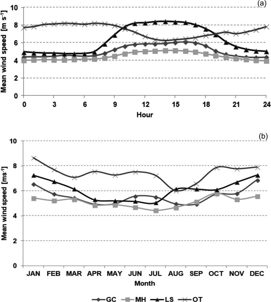
Figure 2 Hourly (a) and monthly (b) mean wind speed (m s-1) for study sites at 10 m above ground level.
Table 3 shows monthly shape and scale parameters and wind power density for each site at 30, 60, and 90 m above ground level. Weibull distribution parameters usually vary from site to site, as in this case. These results indicate that the mean shape parameter for the region lies within the range of 1.57 (GC) and 2.49 (OT). The k parameter exhibited a slight inter-monthly variability, although discontinuous peaks occurred. Monthly k values ranged from 1.30 to 1.87 for GC, from 1.57 to 1.78 for MH, and from 1.60 to 1.95 for LS. For the offshore site, monthly k values were always above 2, ranging from 2.16 to 2.81.
Table 3 Monthly Weibull parameters (k and c) and wind power (W m-2 ) for all sites at different heights. AVG: Average.
| Site | Variable | JAN | FEB | MAR | APR | MAY | JUN | JUL | AUG | SEP | OCT | NOV | DEC | AVG |
|---|---|---|---|---|---|---|---|---|---|---|---|---|---|---|
| GC | k | 1.87 | 1.89 | 1.54 | 1.55 | 1.44 | 1.30 | 1.48 | 1.33 | 1.43 | 1.63 | 1.67 | 1.66 | 1.57 |
| c (30 m) | 8.53 | 8.16 | 6.79 | 6.31 | 6.18 | 6.86 | 6.65 | 5.98 | 6.31 | 7.53 | 7.57 | 8.14 | 7.08 | |
| Pv (30 m) | 543 | 469 | 364 | 289 | 311 | 382 | 368 | 334 | 336 | 456 | 442 | 553 | 404 | |
| c (60 m) | 9.47 | 9.06 | 7.54 | 7.00 | 6.86 | 7.62 | 7.37 | 6.63 | 7.00 | 8.36 | 8.40 | 9.03 | 7.86 | |
| Pv (60 m) | 743 | 642 | 499 | 395 | 426 | 521 | 501 | 456 | 459 | 618 | 604 | 758 | 552 | |
| c (90 m) | 10.01 | 9.58 | 7.97 | 7.40 | 7.26 | 8.07 | 7.80 | 7.02 | 7.40 | 8.84 | 8.88 | 9.55 | 8.32 | |
| Pv (90 m) | 878 | 759 | 589 | 466 | 503 | 616 | 594 | 541 | 542 | 731 | 714 | 896 | 652 | |
| MH | k | 1.75 | 1.63 | 1.62 | 1.70 | 1.70 | 1.79 | 1.6 | 1.6 | 1.63 | 1.6 | 1.57 | 1.63 | 1.65 |
| c (30 m) | 7.14 | 6.42 | 6.13 | 5.56 | 5.18 | 5.00 | 5.41 | 5.43 | 5.79 | 6.95 | 6.62 | 7.1 | 6.06 | |
| Pv (30 m) | 347 | 280 | 246 | 171 | 138 | 116 | 173 | 175 | 205 | 366 | 327 | 379 | 244 | |
| c (60 m) | 8.50 | 7.62 | 7.26 | 6.54 | 6.06 | 5.77 | 6.2 | 6.36 | 6.81 | 8.19 | 7.81 | 8.35 | 7.12 | |
| Pv (60 m) | 576 | 464 | 401 | 278 | 219 | 178 | 257 | 281 | 334 | 587 | 530 | 605 | 393 | |
| c (90 m) | 9.33 | 8.35 | 7.95 | 7.15 | 6.60 | 6.23 | 6.68 | 6.94 | 7.43 | 8.95 | 8.52 | 9.1 | 7.77 | |
| Pv (90 m) | 756 | 605 | 522 | 363 | 283 | 225 | 319 | 368 | 434 | 759 | 689 | 775 | 508 | |
| LS | k | 1.94 | 1.83 | 1.72 | 1.71 | 1.95 | 1.72 | 1.76 | 1.60 | 1.70 | 1.76 | 1.80 | 1.84 | 1.78 |
| c (30 m) | 9.50 | 8.65 | 7.83 | 6.65 | 5.94 | 6.21 | 6.05 | 7.39 | 7.78 | 7.85 | 8.75 | 9.44 | 7.67 | |
| Pv (30 m) | 723 | 582 | 469 | 290 | 175 | 234 | 209 | 440 | 468 | 457 | 615 | 751 | 451 | |
| c (60 m) | 10.19 | 9.27 | 8.39 | 7.13 | 6.36 | 6.65 | 6.49 | 7.92 | 8.34 | 8.42 | 9.38 | 10.12 | 8.22 | |
| Pv (60 m) | 892 | 716 | 577 | 357 | 214 | 287 | 259 | 542 | 576 | 565 | 757 | 925 | 556 | |
| c (90 m) | 10.57 | 9.62 | 8.71 | 7.40 | 6.60 | 6.91 | 6.73 | 8.22 | 8.66 | 8.74 | 9.73 | 10.50 | 8.53 | |
| Pv (90 m) | 990 | 795 | 645 | 399 | 240 | 321 | 288 | 606 | 645 | 631 | 845 | 1033 | 620 | |
| OT | k | 2.81 | 2.16 | 2.32 | 2.28 | 2.61 | 2.58 | 2.38 | 2.56 | 2.39 | 2.65 | 2.76 | 2.34 | 2.49 |
| c (30 m) | 11.11 | 9.85 | 9.44 | 9.99 | 9.53 | 9.89 | 9.23 | 7.89 | 8.58 | 10.21 | 10.23 | 10.67 | 9.72 | |
| Pv (30 m) | 862 | 719 | 596 | 716 | 566 | 637 | 547 | 325 | 438 | 690 | 679 | 855 | 636 | |
| c (60 m) | 11.90 | 10.56 | 10.11 | 10.71 | 10.22 | 10.60 | 9.89 | 8.46 | 9.2 | 10.94 | 10.96 | 11.44 | 10.42 | |
| Pv (60 m) | 1059 | 886 | 732 | 883 | 698 | 785 | 673 | 401 | 540 | 849 | 835 | 1054 | 783 | |
| c (90 m) | 12.36 | 10.96 | 10.50 | 11.11 | 10.60 | 11.00 | 10.26 | 8.78 | 9.55 | 11.36 | 11.38 | 11.88 | 10.81 | |
| Pv (90 m) | 1187 | 990 | 820 | 985 | 779 | 879 | 751 | 448 | 604 | 951 | 935 | 1181 | 876 |
The scale parameter showed a clear temporal pattern characterized by lower values in winter and higher in summer (Table 3). At an intermediate height (60 m), monthly c values (m s-1) ranged from 5.8 to 8.5 for MH, from 6.4 to 10.2 for LS, from 6.7 to 9.5 for GC, and from 8.5 to 12 for OT.
According to Elliott et al. (1987), mean wind power density (calculated by averaging monthly values) was graded as fair/moderate for MH (244 W m-2 at 30 m, 393 W m-2 at 60 m), good for sites GC (404 W m-2 at 30 m, 552 W m-2 at 60 m) and LS (451 W m-2 at 30 m, 556 W m-2 at 60 m), and excellent for the offshore site at both height levels (636 W m-2 at 30 m, 783 W m-2 at 60 m), (Table 3). Wind power density for sites GC, LS and OT was graded as good and excellent during winter and summer, respectively, at both 30 and 60 m; for the remaining site (MH), wind power density was fair in winter and good in summer. At 90 m, mean wind power density reached 508 W m-2 for MH, 620 W m-2 for LS, 652 W m-2 for GC, and 876 W m-2 for OT.
Solar PV Potential
Figure 3 shows monthly mean solar radiation and mean cloud cover for the three sites monitored. Solar radiation ranged from 163 W m-2 (June) to 556 W m-2 (December) for GC, from 195 W m-2 (June) to 467 W m-2 (January) for MH, and from 212 W m-2 (June) to 530 W m-2 (January) for LS. In this study area, with a latitude ranging from 38°38 to 39°30S, mean sunshine duration varied from 8.28 h in June to 13.85 h in December. Peak values occurred at about 13:00 local time.
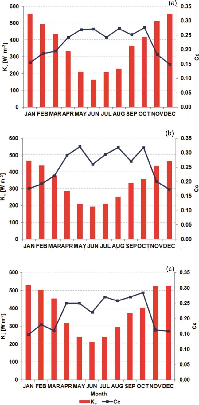
Figure 3 Monthly mean solar radiation (watt hours per square) and monthly mean cloud cover for sites GC (a), MH (b), and LS (c).
Cloud cover varied between sites. Mean cloud cover was 0.218, 0.225, and 0.253 for LS, GC and MH, respectively. The intra-annual behavior of cloud cover for all sites followed a pattern opposite to that of solar radiation intensity (Figure 3). Thus, in winter, and to a lesser extent in intermediate seasons, the monthly mean cloud cover was close to 0.30, whereas in summer it did not exceed 0.20.
Figure 4 shows the evolution of cloud cover and ONI (Oceanic Niño Index) for MH between 2010 and 2016. MH was selected for this analysis because it had the longest solar radiation recording period. During that period, two opposite events (El Niño and La Niña) varying in intensity level were identified. The most significant episodes were one moderate La Niña (from September 2010 to January 2011) and one strong El Niño (from November 2014 to February 2015). Extreme cloud cover and ONI values were seemingly out of phase with each other. As regards the moderate La Niña episode, clear-sky conditions were observed with cloud cover values ranging from 0.12 to 0.18 only; after three months of the strong El Niño episode, a peak of 0.45 was recorded.

Wave Potential
The study area is exposed to waves generated by local winds (Figure 2), mostly in spring. In winter, the longest periods were mainly associated with waves from the Atlantic Ocean. Mean Hs for the study period was 0.78 m, with a standard deviation of 0.14 m (monthly values). Figure 5 shows monthly averages of Hs, T and wave power for the study site. Peak monthly Hs values were recorded in spring-summer; in May, Hs was also high. In contrast, winter recorded the lowest Hs values, with more than 50 % of waves smaller than 0.5 m in height, and with long periods of more than 8 s.

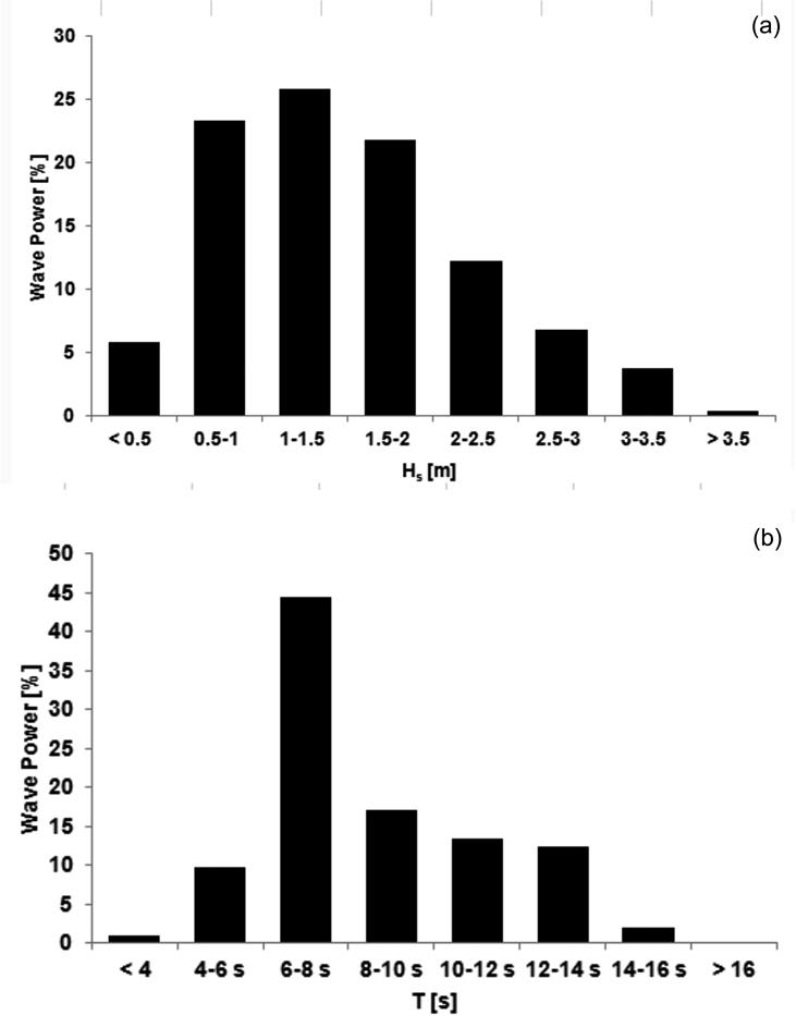
Mean T for the whole period was 8 s. In general terms, T seemingly followed a trend opposite to that of Hs (Figure 5). This is an important observation, since the resulting wave power is a function of both Hs and T (Eq. 7). Thus, the monthly mean wave power peaked in September and November (4.6 kW m-1), followed by May (3.8 kW m-1) and January (3.3 kW m-1) (Figure 5). Mean wave power was 2.8 kW m-1. Figure 6 shows the percentage of wave power at various intervals of Hs (0.5 m) and T (2 s). The maximum wave power was recorded at 1-1.5 m (25.8 %) and 4-6 s (23.3 %).
Power Load Demand versus Renewable Sources
Table 4 shows the average monthly consumption for the three cities of interest (Bahía Blanca, Monte Hermoso and Pedro Luro). These cities differ in many ways, including main economic activity, population size, etc. The Study area section and Table 1 provide details on electricity consumption (e.g., annual consumption level and number of users for each main economic sector) for the three cities. In all cases, the highest consumption occurs during summer, mainly in January, with increases of 15, 55 and 17 % over the minimum values for Bahía Blanca, Monte Hermoso and Pedro Luro, respectively (Table 4). This behavior is most pronounced in the coastal city of Monte Hermoso, resulting from the seasonality of tourism (sun and beach product).
Table 4 Average monthly consumption (MW h) for the three cities.
| JAN | FEB | MAR | APR | MAY | JUN | JUL | AUG | SEP | OCT | NOV | DEC | |
|---|---|---|---|---|---|---|---|---|---|---|---|---|
| Bahía Blanca | 144477 | 126431 | 135976 | 127778 | 135353 | 127483 | 124822 | 127981 | 125808 | 127376 | 123859 | 136271 |
| Monte Hermoso | 4117 | 3294 | 2196 | 1798 | 1872 | 1881 | 2030 | 1932 | 2006 | 1873 | 1831 | 2558 |
| Pedro Luro | 1295 | 1085 | 1162 | 1108 | 1194 | 1217 | 1251 | 1201 | 1127 | 1126 | 1077 | 1265 |
Source: Data provided by Ministry of Energy and Mining, Argentina.
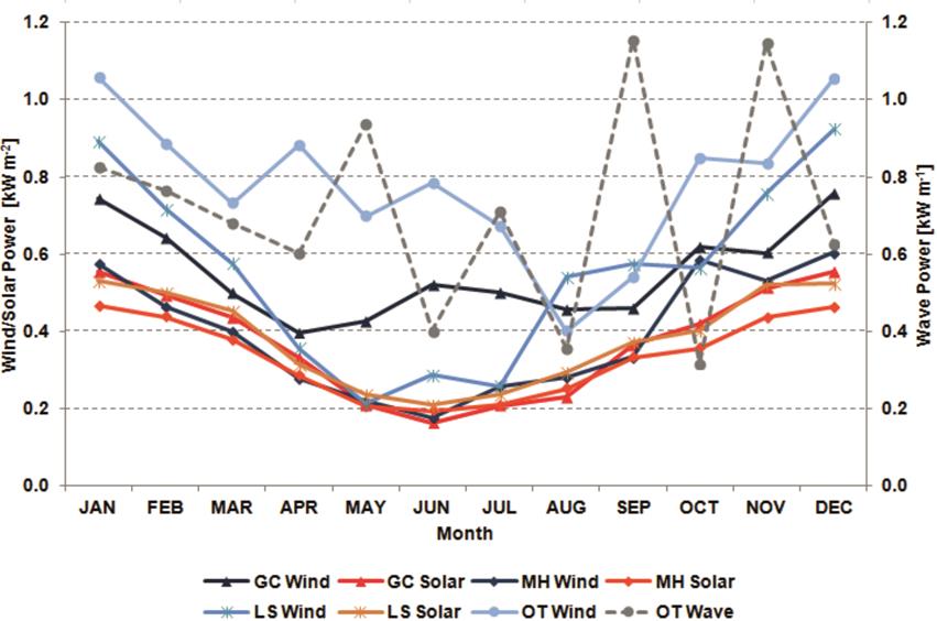
Figure 7 shows monthly wind, solar, and wave power for all sites already considered, to summarize power availability. There is an overall pattern of increasing power levels during summer, particularly when considering wind and solar sources, reaching mean values up to 1.06 kW m-2 (wind at 30 m height, OT) and 0.56 kW m-2 (solar, GC). On average, wind and solar power showed variations of 65 % and 63 % between minimum and peak annual values, respectively. On the other hand, wave power showed a higher (intra-annual) variability.
The Pearson correlation coefficient, which quantifies the similarity between two data sets, was applied to measure the association between electricity load demand and a given power source (wind, solar, and wave) on a monthly basis. The key point is that when considering associations between load demand and power available from renewable sources, the identification of positive correlations is essential.
Figure 8 shows seasonal and annual correlation coefficients between electricity load demand and each source for the three cities. Regarding the wind source, the annual correlation coefficient ranged from 0.05 (Pedro Luro) to 0.52 (Monte Hermoso). However, as expected, some seasonal values yielded higher correlations. For instance, in summer, when consumption rises considerably, correlations were high (and positive) for Bahía Blanca (r = 0.83) and Pedro Luro (r = 0.95) (Figure 8a,c). In contrast, in the case of Monte Hermoso, the correlation was low (Figure 8b) due to the fact that the disproportionate consumption, which is highly concentrated in January (Table 4), differs from the trend of wind power (Figure 7). As regards the solar source, the annual correlation between load demand and solar power ranged from -0.14 (Pedro Luro) to 0.63 (Monte Hermoso). In summer, correlations were high (and positive) for Bahía Blanca (r = 0.88) and Pedro Luro (r = 0.99) (Figure 8a,c), and low for Monte Hermoso (r = 0.15) (Figure 8b), similar to those observed for wind. Finally, wave power was poorly correlated (r < ±0.2) with load demand in annual terms, for the three cities. Seasonal correlations were high, with some exceptions.

Integration of Renewable Sources
Table 5 shows the Pearson correlation coefficients between the different sources at multiple time scales (hourly, daily, and monthly) for all monitoring sites. This coefficient was determined based on mean values. When considering associations between the different sources in search of complementarity options, the identification of uncorrelated or negatively correlated results is essential.
Table 5 Correlation coefficients between the different sources at multiple time scales for all sites.
| Monitoring site | Time scale | Wind co. vs. Solar | Wind co.vs. Wave | Solar vs. Wave | Wind off. vs. Wind co. | Wind off. vs. Solar | Wind off. vs. Wave |
|---|---|---|---|---|---|---|---|
| GC | Hourly | 0.921 | -0.743 | -0.767 | -0.788 | -0.736 | - |
| Daily | 0.410 | 0.101 | 0.289 | 0.167 | 0.142 | - | |
| Monthly | 0.812 | 0.433 | 0.644 | 0.786 | 0.547 | - | |
| MH | Hourly | 0.914 | -0.749 | -0.742 | -0.841 | -0.702 | - |
| Daily | 0.207 | 0.011 | 0.224 | 0.031 | 0.102 | - | |
| Monthly | 0.782 | 0.509 | 0.571 | 0.657 | 0.334 | - | |
| LS | Hourly | 0.918 | -0.673 | -0.714 | -0.831 | -0.728 | - |
| Daily | 0.415 | 0.131 | 0.216 | 0.082 | 0.099 | - | |
| Monthly | 0.937 | 0.456 | 0.646 | 0.466 | 0.549 | - | |
| OT | Hourly | - | - | - | - | - | 0.755 |
| Daily | 0.192 | ||||||
| Monthly | - | - | - | - | - | 0.407 |
Wind co.: continental/onshore wind; Wind off.: offshore wind.
In general, a clear pattern of associations is observed. The correlation between wind (continental/onshore) and solar sources was high and positive for all monitoring sites on hourly and monthly time scales, but weak on a daily time scale. In this study area, both wind and solar power followed a very similar temporal trend at hourly and monthly time scales, meaning these cannot complement each other for combined exploitation. Most of the remaining power source pairs, i.e., wind (continental/onshore) versus wave, solar versus wave, wind (offshore) versus wind (continental/onshore) and wind (offshore) versus solar, showed a high negative correlation at the hourly time scale and a weak correlation (approximately from 0.3 to 0.7) at a monthly time scale, indicating that these may be complementary. In the particular case of OT, correlations were high (and positive) and weak at hourly and monthly time scales, respectively.
DISCUSSION AND CONCLUSIONS
This study conducted an assessment of wind, solar, and wave energy sources in the southwest of Buenos Aires Province (Argentina). The main goal was to assess the feasibility of the energy sources mentioned above by evaluating their potential for electricity production, their relationship with electricity load demand, and the extent of integration between them. To note, no studies are currently available on this subject, not even at the national level. The present study was based on data from four stations: three are located in coastal sites (onshore: GC, MH; offshore: OT); the remaining station (LS) is located in a shallow lake.
As regards the wind source, its characteristics exhibit some spatio-temporal variability across the study area. For instance, the offshore site showed higher wind speed values (annual average = 7.4 m s-1 at 10 m height) vs continental/onshore sites for the whole year. In addition, onshore sites (GC and MH) were characterized by moderate turbulence (intensity), whereas the offshore site (OT) exhibited low turbulence (Genchi et al., 2014); this low turbulence at sea leads to increased power effectiveness. Among continental/onshore sites, LS showed the highest wind speed (annual average = 6.1 m s-1 at 10 m height), followed by GC and MH, in agreement with the available wind speed maps (e.g., AWS Truepower). From a temporal perspective, a similar pattern was observed across the study area, with wind speed reaching peak values from October to February and the lowest during winter. This evidences spatio-temporal variability in power availability. Thus, according to Elliott et al. (1987), wind power density for sites GC, LS and OT was graded as good and excellent during winter and summer, respectively, at both 30 and 60 m height; in the remaining site (MH), wind power density was fair in winter and good in summer.
As regards the solar source, the amount of solar radiation in the study area is typical of subtropical latitudes, ranging approximately from 200 W m-2 (January) to 500 W m-2 (December). The spatial variability of solar radiation depends more on cloudiness than on latitude, since the study area comprises a small latitudinal range (≈ 1°). Cloud cover was higher in MH (annual average = 0.25) than in the remaining inland sites, in response to the influence of coastal location on climate. From a temporal standpoint, cloud cover in all sites increased in winter, and to a lesser extent in intermediate seasons, reaching values close to 0.30, whereas in summer it did not exceed 0.20. The latter exacerbates the latitudinal effect of solar radiation. It should be mentioned that a long-term analysis revealed that cloud cover may be influenced by El Niño-Southern Oscillation variability.
In the case of the wave source, mean Hs and T for the whole period were 0.78 m and 8 s, respectively. Wave power fluctuated throughout the year; monthly mean wave power reached peak levels in September and November (4.6 kW m-1), followed by May (3.8 kW m-1) and January (3.3 kW m-1). Our results are consistent with those reported by Lanfredi et al. (1992), who determined wave power in the SE of the Buenos Aires Province (nearshore), with mean values ranging between 2.3 and 7.5 kW m-1. Therefore, the study site is characterized by a low wave power relative to other areas. However, considering the well-known advantages of electrical power generation from waves, it is reasonable to assume that even at this low potential, the exploitation of wave power may be significant and, therefore, an evaluation of wave energy conversion becomes important. Thus, recent studies focused efforts on evaluating the feasibility of installing wave energy converters also in low-energy seas (e.g., Iuppa et al., 2015; Naty et al., 2016; Foteinis and Tsoutsos, 2017).
Many studies focused on electricity load demand revealed that load demand is a non-stationary process that depends on human activities and weather conditions (Al-Hamadi and Soliman, 2004). The three cities considered in this study (Bahía Blanca, Monte Hermoso and Pedro Luro) show differences, for example, in main local economic activities and population size, which affect electricity consumption. These cities showed the highest consumption in summer, being more marked in Monte Hermoso, related to its climate-driven primary activity (sun and beach tourism). Increased consumption levels were accompanied by generalized power outages in recent summers, due to the widespread use of cooling appliances. In winter, there is a slight rise in consumption at Monte Hermoso and Pedro Luro, partly due to an increased use of electrical heating devices to mitigate the limitations of natural gas services.
In general, the highest power levels were observed in summer months, coinciding with the peak energy demand. On the other hand, on an hourly basis, the highest wind and solar power levels occur during daylight hours, i.e., when people are at home and active. In order to measure the association between electricity load demand and the power sources studied, the Pearson correlation coefficient was applied on the monthly analysis. To note, annual correlation coefficients were not very high, partly because both load demand and power sources naturally follow their own dynamics. The highest correlations corresponded to wind and solar sources for Bahía Blanca and Monte Hermoso. Seasonally, several correlation coefficients were higher vs annual correlation coefficients. For instance, in summer, when electricity consumption is high, correlations related to wind and solar sources were high and positive for Bahía Blanca and Pedro Luro, but low for Monte Hermoso as a result of intense electricity consumption in January; correlations related to wave power were high for Bahía Blanca and Monte Hermoso but moderate for Pedro Luro. Therefore, the peak energy demand in summer may be supplied alternatively by different renewable sources. Our results should be deemed preliminary due to the lack of detailed data on electricity load demand.
The Pearson correlation coefficient for assessing relationships between renewable sources has been successfully applied in similar studies (e.g., Widén et al., 2015; de Oliveira Costa Souza Rosa et al., 2017) due to its simplicity and effectiveness. In the present study, this coefficient was applied at multiple time scales (hourly, daily, and monthly) for all monitoring sites. As regards the association between wind and solar sources, correlation coefficients were high and positive for all monitoring sites at hourly and monthly time scales; in this study area, unlike other regions of the world, both wind and solar power follow a very similar temporal trend, characterized by highest power levels during daylight hours and in the summer, meaning that these cannot complement each other for a combined exploitation. However, most of the remaining power source pairs — wind (continental/onshore) versus wave, solar versus wave, wind (offshore) versus wind (continental/onshore) and wind (offshore) versus solar — showed a high negative correlation on an hourly time scale and a weak correlation on a monthly time scale, resulting in promising results in terms of complementarity.
This study will support a larger role of renewable electricity sources in electricity production, contributing to achieve sustainability goals. Today, four wind farm projects within the program “RenovAr - Programa de Energías Renovables” of the Ministry of Energy and Mining are under development in the southwest of Buenos Aires Province, making of wind the only growing renewable energy technology.
This analysis is a preliminary approximation, but given the promising results obtained, will continue by exploring other potential power sources such as biomass for energy generation. In future work, key research lines will focus on energy production technologies, exploring their benefits and limiting factors.

