


 nueva página del texto (beta)
 Inglés (pdf)
 Artículo en XML
 Referencias del artículo
 Enviar artículo por email
 Citado por SciELO
  Similares en
SciELO
Similares en
SciELO 
 Permalink
Introduction
Many Digital Elevation Models (DEMs) are derived from LiDAR (Light Detection And Ranging) data. Two main types of DEM are produced in order to study the Earth's surface: a Digital Surface Model (DSM) that corresponds, excepting abnormal registers, to the first returns of the LiDAR threedimensional points cloud that contains all the features of the Earth's surface (ground, vegetation and constructions); and a Digital Terrain Model (DTM) that takes into account the last returns and that fits the bare earth surface. Nevertheless, the last returns do not always reach the bare earth surface if the radar beam encounters an obstacle. If the filters fail to extract the terrain, polygons and/or reference points are manually introduced. Depending on the interpolation method used, the resulting DTM presents artifacts such as triangular facets that do not correspond to an objective representation of the bare earth. The present paper proposes a method of correcting these artifacts, since accurate high-resolution information is required for precise calculations. It falls into four sections: a) a general survey of LiDAR DTM generation and associated artifacts; b) a description of the area used as an example of the treatment; c) the method developed for the type of artifacts detected in the study area; d) a discussion of the results.
GENERATION OF LiDAR DIGITAL TERRAIN MODELS
The point cloud laser scanner obtained from the LiDAR survey is commonly segmented by using different filters to extract the ground surface or the above-ground features (Pfeifer et al., 1998; Axelsson 1999, 2000; Sithole, 2001; Vosselman, 2000; Vosselman and Maas, 2001; Roggero, 2001; Brovelli et al, 2002; Wack and Wimmer, 2002; Zhang et al., 2003; Vosselman et al., 2004; Zhang and Whitman, 2005). The American Society for Photogrammetry and Remote Sensing has developed the Lidar Archive Standard (LAS) as an option for binary data exchange for LiDAR point data records; this allows different hardware and software to manage a common format in order to segment and classify all the returns. These binary data consist of a public header block, variable length records and point data records. Each point of the point cloud in the LAS format (American Society for Photogrammetry and Remote Sensing, 2008) has different classified information. Among the plans that can be extracted from the point cloud are the surface and terrain. If the goal is to obtain a bare-earth terrain model, at least the following four categories must be defined: ground, above-ground objects (trees, buildings, bridges, etc.), water and noise.
Software packages use automatic and manual edition in order to obtain the bare earth surface. For instance, the main algorithms used by the ALDAPAT software (Zhang and Cui, 2007) are based on the elevation threshold with expanding window (Zhang and Whitman, 2005), the progressive morphology (Zhang et al., 2003) for one and two dimensions, the maximum local slope (Vosselman, 2000), the iterative polynomial fitting, the polynomial 2-surface filter or an adaptive triangular irregular network (TIN) (Axelsson, 2000). Generally, the absolute minimum and maximum elevations in a dataset are used in order to define an elevation scale. Following this logic, an algorithm developed by one of the authors (Parrot, 2013a) proposed an easier procedure that directly uses the point cloud data to generate a Digital Terrain Model. The calculation must take into account the smallest possible pixel size circumscribing the buildings in the study area. This size may differ from one zone to another and it is necessary to accurately measure any regional changes to ensure that the last return of the studied local area is the real signature of the bare earth surface. The algorithm developed to address this problem makes locally a number of tests with different pixel size to generate an image of the bare earth surface. As shown in the example (Figure 1), this procedure avoids the use of polygons to define the altitude of the land under the buildings. A similar treatment has been developed to estimate the canopy cover (McGaughey, 2009 and 2014), but in this case the operation uses two variables: height breaks and cell size. In order to obtain a significant cover assessment, the cell size must be larger than individual tree crowns.

Figure 1 Digital Surface Model (dsm) reported onto the Digital Terrain Model (dtm) (bare earth surface using a colored hypsometric scale [green to red]) generated from the point cloud.
Adaptive filters attempt to identify or delineate terrain type or terrain cover according to the study requirement. These algorithms codify around 90% of the data set, but the remaining points need to be classified by manual editing. Manual edition involves visually assessing, eliminating and/or adding points using ancillary data such as the imagery collected in the LiDAR survey; it also involves photogrammetric imagery, hill shades, contours, and polygon extraction to remove the non-bare-earth points.
LiDAR DTM ARTIFACTS
The nature and density of vector information when passing to raster products generate artifacts in derived products, and linear features will lose their integrity. In order to generate continuous surfaces that conserve linear terrain features, the common photogrammetric techniques consist of adding break lines and lines with three-dimensional vertices and three-dimensional polygons. Among other photogrammetric techniques, lidargrammetry (Fowler et al., 2007) is based on pseudo stereo pairs obtained from an image of intensity plus the elevation data, and it allows visual selection of the ground features. The resulting LiDAR DTM remains with artifacts such as triangular facets and irregular altitudes in the river profile. This is particularly clear for points captured along a shoreline in relation to the presence of vegetation and natural ground roughness. Furthermore, random returns above the water surface may occur without any relationship to elevation values. In this last case, classification uses the hydrologic enforcement technique that consists of adding break lines or polygons along lake edges, river banks or coastal shorelines, giving a constant elevation to a flat water surface. Nevertheless, the slope downstream remains unsolved.
These defects lead to miscalculations when modeling and simulating various hydrological processes such as floods. In the following sections, the correction of triangular facets and river altitude is presented as well as the root-mean-square error (RMSE) evaluation of the previous and resulting models.
DATA USED AND STUDY AREA
The ASCII data (_mt.xyz) provided by INEGI (2013) are transformed to .raw raster format by using the algorithm Transf_ascii_xyz_dem_lidar (Parrot, 2013b). First, this algorithm searches the minimum and maximum of UTM coordinates in order to define the size of the resulting file according to the pixel size that in these data is 5 m. Moreover, information provided by the ASCII file allows identification of the decimal digit of the z value that indicates whether the altitude is measured in meters, decimeters, centimeters or millimeters, and this allows transformation of the float values as integers without loss of hypsometric precision. In the present case the resulting DTM has centimetric vertical resolution. The algorithm transforms the ASCII data (_mt.xyz) provided by INEGI in a raster file i, j, z (where i and j correspond to the lines and columns; z remains as the altitude value).
The program generates not only a raster file, but also an ASCII file that can be used by Geographic Information Systems (GIS).
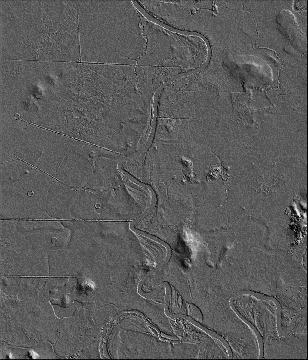
The study zone corresponds to a fluvial plain to the west of Coatzacoalcos River (Veracruz State). This fluvial plain (between 0 and 10 m a.s.l.) is characterized by dynamic changes associated with lateral migration of the river banks, deltaic subsidence, marine transgression and diapirism (Figure 2).

METHOD
Quality control
The artifacts concern mainly triangular facets in hills and particularly incoherent altitude values for river surfaces resulting from missing altitude values in an area of dense vegetation. Moreover, water bodies present specular effects, so that the amount of energy of the laser beam returned to the sensor is very low and altitude estimations are imprecise.
The quality control can indicate possible data problems displayed as shifts or scaling errors. Sometimes the creation of the corresponding contour lines from LiDAR data allows mismatches or noise points to be distinguished. These points correspond to spikes or wells scattered onto the true bare earth surface.
Another way consists in developing an absolute accuracy assessment that compares the LiDAR product with ground control points (Ivanov and Kruzhkov, 1992; Bolstad and Stowe, 1994; Wechsler, 1999). However, such RMSE techniques present drawbacks. Florinsky (2012) estimates that "it is unreasonable to consider the reference DEM as a correct model".
We assess the degree of improvement by measurement before and after the proposed treatment. Measurement of the accuracy of DEMs is based, among other things, on the calculation of the Root Mean Square Roughness (Rq or RMSR) as well as of the RMSE. Rq is the square root of the sum of the squares of the height that can be calculated line by line, column by column or by use of the whole image. The formula used in the case of the whole image is as follows:

where  corresponds to the mean value of the altitudes defined as,

m the number of lines, n the number of columns and z the altitude of each point i, j.
Meanwhile, the RMSE is calculated as follows:

where ξ is a point of elevation from the studied elevation model, χ the value of a corresponding point on a reference surface and N the number of sample points. Felicísimo (1994) suggested generation of the reference surface by consideration of the hypsometric values of the four cardinal neighbor pixels of each LiDAR DTM pixel. Since this process is applied to all DTM pixels, it is also possible to calculate the arithmetic mean and standard deviation of these differences.
Enhancement treatment
The main lines of the improving treatment concern firstly the elimination of triangular facets observed locally and essentially the irregular roughness of the drainage network surfaces.
a) Triangular facets
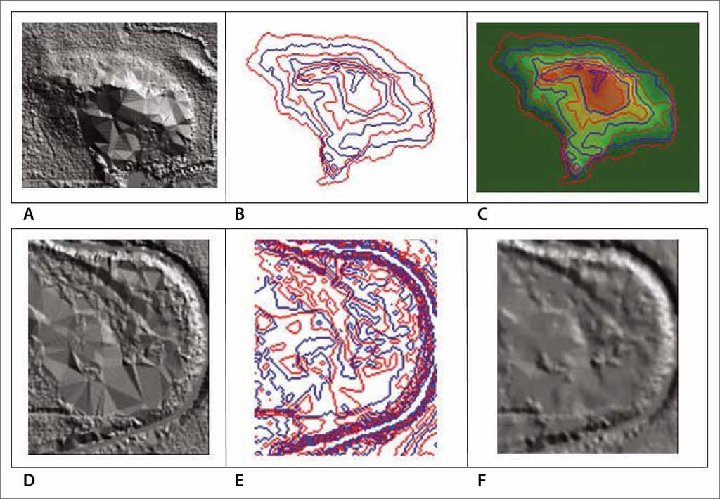
The presence of local TIN results from interpolation and also from lidargrammetry methods (Fowler et al., 2007; Maune, 2007) that allow improbable elevations to be eliminated by human interpretation. Even if the remaining elevations are derived from the LiDAR data themselves, such an operation creates small areas without altitudinal information, areas that fill the triangulation (Figure 3).

The proposed method to locally improve landforms consists in taking into account the three vertices of the triangular polygon to generate local contour lines that allow the morphology to be reconstructed by means of a simple interpolation (Dilat_curves, Parrot, 2005).
The area to be reconstructed is extracted from the LiDAR DTM, and the corresponding contour lines provided by the first step of the treatment are reported in an 8 bits image (Figure 4). This iterative treatment consists of extraction of all the pixels whose altitude equals or is lower than the altitude of the researched contour line; the perimeter of the generated surface corresponds to the contour line. Each extracted contour line that has a gray tone value according to the hypsometry is eventually corrected in order to obtain 8 vicinity curves (Figure 4B). Two MS-DOS executable programs are used (Extra_courbes4.exe, Parrot, 2004; Net_curve.exe, Parrot, 2003a). Then, a contour line dilation technique (Taud et al., 1999) uses a table of correspondence between a gray tone value and its altitude, and the local improved area (Figure 4C) is reincorporated at its place in the LiDAR DTM (Pegaim.exe, Parrot, 2003b). The same process is applied to fluvial forms (Figure 4D, 4E and 4F) and to zones that present the same artifacts.
Drainage network surfaces
As mentioned above, points obtained all around water bodies, and mainly when they correspond to a drainage network, vary strongly and abruptly in altitude according to the presence of vegetation of different heights and the presence of natural ground roughness in relation to meander scrollbars.
In general, manual drawings are proposed for the definition of water polygons used to assign an elevation value to the water surface; such a procedure is called hydrologic enforcement. The method presented here is partly based on such an approach, but takes especially into account the slope downstream.
In a first step, it is necessary to extract the river surfaces that will play the role of a mask to be used in the procedure. This extraction is based not on polygon digitization but on automatic extraction provided by the software TLALOC_V2 (Parrot, 2015) that defines local hypsometric slices. Then, the skeleton of the mask of the drainage network segment is obtained by means of a thinning method (O'Gorman, 1990). Endpoints of this skeleton are used to calculate the altitude of all the successive pixels that describe the one-pixel- width skeleton of the river. The altitude of the two endpoints is firstly assessed by the original DTM and these values have been controlled in the field. The altitudinal path corresponds to the difference of altitude between the two endpoints divided by the number of pixels belonging to the skeleton river. In fact, the number of intervals is taken into account and this number is equal to the number of pixels minus one. At this stage, the problem consists then in assigning a hypsometric value to the points that are in the mask. The treatment (Figure 5) attributes an altitude value to each mask point when this point has at least, inside a 3 x 3 pixel, a cardinal neighbor pixel that registers an altitude value. When two or three cardinal neighbors present a hypsometric value, the mean is adopted for the pixel. At the beginning of the procedure, only the pixels belonging to the skeleton river have a hypsometric value. The treatment is not a sequential treatment and at each step the resulting values must be registered in a provisional 4 byte image and recovered in order to continue with the treatment. The procedure stops when the altitudes of all the pixels of the river mask have been defined and the result is superposed onto the original LiDAR DTM.

RESULT AND DISCUSSION
The LiDAR DTM resulting from the local transformations presented above is shadowed in order to visually check the modifications generated by the treatment (Figure 6). In addition, as mentioned above, the RMSE calculation can be used to underline the slight differences observed between the two DTMs.
The RMSR of the original LiDAR DTM is 1.431 when calculating line by line, or 1.418 when calculating column by column or 1.759 when the whole image is taken into account. In the case of the transformed DTM, these RMSR values are, respectively, 1.411, 1.396 and 1.746; this result shows that the roughness decreases slightly in relation to the small surfaces that have been transformed. Moreover, the RMSE of the original LiDAR DTM calculated by the Felicísimo treatment (1994) is 0.0826 with a standard deviation of 0.0701, whereas for the transformed DTM this value is 0.0774 with a standard deviation of 0.0634. All these values reflect the positive aspect of this method of improvement. It is also interesting to compare the two DTMs by calculating the RMSE while taking into account the original DTM as a reference. The resulting values are as follows: RMSE = 0.179999, β1 = 1.001894 and β0 = -0.022658; this demonstrates that the two products are globally similar.
The RMSR and RMSE of elevation applied to the corrected areas emphasize locally the enhancement. For instance, in the area of the hill (Figure 7a, 7b, 7c and 7d) the RMSE of the original DTM is 0.067 and becomes 0.012 in the reconstructed form. These results and the illustrations reported in Figure 7 show the enhancement behavior. Triangular facets disappear and portions of the drainage network extracted by means of a TLALOC software (Parrot, 2006) function and reported on the DTM aspect demonstrate the process accuracy. In the case of meanders, these values are 0.101 for the original landform and 0.034 in the case of corrected shape. All these values are reported in Table 1.

Figure 7 dtm Hillshade: A, original dtm, B, corrected dtm. Aspect and drainage network extraction. C, original dtm and D, corrected dtm.
Table 1 rmsr and rmse for dtms.
| RMSR | RMSE | St. deviation | RMSE between DTMs | |
|---|---|---|---|---|
| Original LiDAR DTM Hill | 2.309 | 0.067 | 0.052 | 0.778 |
| Reconstituted Hill | 1.783 | 0.012 | 0.011 | |
| Original DTM Meander | 1.079 | 0.101 | 0.082 | 0.181 |
| Recalculated meander | 0.996 | 0.034 | 0.028 |
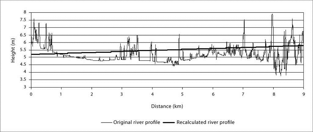
The small decrease reported in this table has to be related to the corrected artifact areas that represent only 5.05% of the DTM (1.66% for meanders and hills, 3.39% for the river surface). As clearly shown by the modifications registered at the level of the river surface (Figure 8 and 9), the RMSR and RMSE decrease is not related to local smoothing but to the selected elimination of artifacts.

Depending on the type of topography, the grid density and the interpolation techniques (Aguilar et al., 2005), different portions of the DEM may have a distinct accuracy. In relation to the increase in slope (Felicísimo, 1995), geometric artifacts occur in mountainous areas. The stronger the relief, the greater the difference (Carlisle, 2005; Fisher and Tate, 2006; Cárdenas et al., 2013).
CONCLUSION
In this paper, we have presented approaches that allow detection and elimination of artifacts and reconstruction of the shapes in order to obtain a surface representation closer to the original terrain.
The use of Digital Elevation Models requires great accuracy, especially when extracting morphometric variables from the DEM surface or when doing different types of simulation such as flooding (Ramírez and Parrot, 2015). There is a need not only for good accuracy but also for a document that does not contain artifacts or biases that diminish the quality of the treatment and distort the representation of the Earth's surface. For these reasons, specific treatments are essential for improved DEMs.

