Artículos

 

Main determinants of tenure choice in Spain: cross–analysis of distinct city sizes

 

Melchior Sawaya Neto*

 

* Doctor en Economía, Departmento de Economía Aplicada, Universidad Autónoma de Barcelona, España. E–Mail: melchior_sawaya@yahoo.com.br

 

Fecha de recepción: agosto de 2006.
Fecha de aceptación: septiembre de 2006.

 

Resumen

La mayoría de los gobiernos diseñan políticas de vivienda homogéneas para todo el territorio nacional sin considerar diferencias en las preferencias económicas de los hogares localizados en ciudades con distintos tamaños. El problema con esta práctica radica en que los hogares localizados en las grandes ciudades probablemente presentan restricciones presupuestarias más fuertes que aquéllos de localidades más pequeñas, dado los mayores niveles de precios de vivienda y peores condiciones de accesibilidad presentes en las ciudades grandes. Con el fin de analizar estas cuestiones fue desarrollado un grupo de modelos de elección discreta con vistas a representar las preferencias de los hogares en ciudades españolas de distintos tamaños: grandes, medias y pequeñas. El resultado demuestra interesantes diferencias en los parámetros estimados para grupos que suelen ser objetos de políticas de vivienda, tales como los hogares comandados por personas jóvenes o compuestos por una única persona. La no consideración de dichas diferencias en parámetros puede causar serios problemas de no participación en programas de gobierno.

Palabras clave: decisión en la elección de tenencia, indicadores de accesibilidad, diferencias en los parámetros estimados, y ciudades de distintos tamaños.

 

Abstract

Many governments design homogeneous housing policies for the whole country without considering differences in economic preferences of households living in cities with distinct sizes. The problem with this practice is that households in larger localities may face stronger budgetary restrictions than those living in smaller ones because of higher housing prices and worse affordability conditions. To deal with this issue a set of tenure choice models are estimated to represent the households' preferences in Spanish cities of different sizes: big, medium or small localities. The results show interesting differences in parameter estimates for groups usually object of public policy such as young household heads and single member families. Disregarding these differences can cause serious problems of non–participation in government programs.

Key words: tenure choice decision, affordability indicators, differences in parameters estimates and cities with distinct sizes.

 

Introducción

The main purpose of this work is to extend the knowledge about the determinants of housing tenure choice in Spain. Thus, distinct geographical sub–divisions will be employed in the analysis, such as: the whole country and large, medium and small city markets. The aim is to investigate the most relevant causes that make an individual or household select a determined sort of tenure and understand how the parameter estimates differ within equations. The methodological procedure of using cities with increasing sizes allows the study of tenure choice in environments with great difference between important parameters, due to the fact that housing prices, income, and demographic variables may differ substantially as the cities changes their sizes.

It is interesting to stress that the knowledge of consumers' preference is a fundamental factor to the success of any housing policy. In theoretical terms, it is very plausible that the housing consumers' economical preferences differ among cities of distinct sizes: the utility functions, used to describe preferences, may be affected unevenly by the same explanatory variable depending in which environment the consumer is located. For instance, monetary variables seems to impact more on the probabilities of homeownership of people living in big cities than those living in small or medium localities. Thus, if a country is thinking about implementing housing policies it may be interesting firstly to know the differences in preferences of possible housing consumers object of policy.

In theoretical terms some assumptions will be tested, introduced by the neoclassical housing economic theory, regarding the importance of relative prices and income in the determination of which sort of tenure to choose. Following the aforementioned theory, the relative price difference among the rental and property sectors flow prices is the main mechanism upon which the decision makers take or base their housing choices. Nevertheless, it is important to stress that not only relative prices affects the demand for housing and tenure choice but also other affordability variables play an important role.

Affordability indicators are variables or series designed to represent various aspects of the demand for property or rental houses such as the ability of housing consumer to save money in order to face the required down payments and closing costs needed to obtain mortgage loans. They represent a combination of monetary variables which traditionally appears alone in demand equations. Thus, some important indicators, employed by this sort of analysis are: 1) the housing expenditure to income ratio; 2) the stock price to income ratio.

Thus, the goals of this work can be summarized by:

1) The empirical analysis of the main factors that affects the tenure choice in Spain;

2) The study of regional differences in parameters.

The work starts with a characterization of some basic theoretical results regarding the main features of the demand for housing services and their connection with the tenure choice decision. Secondly, the discrete choice model will be introduced and discussed. Finally, the empirical analysis of the tenure choice equations will be delineated.

 

2. The demand of housing services. Tenure choice and affordability indicators

The main objective of this section is to discuss how essential features of housing demand and tenure choice modelling are commonly treated in the literature. Also, the role of affordability indicators in tenure choice and demand analysis will be debated. As usual, in any demand analysis, the characterization of the model depends on the specification of the utility function and the budget constrains: these expressions assume some special features in this market, see (Deaton and Muellbauer, 1991, pp. 97–108) and (Olsen, 1986, pp. 989–995), following the durable properties of the housing good.

Starting with the utility function, the options of the consumer are aggregated into two broad groups of commodities, h (housing services) and X (a composite index of other goods). The period in which decisions can be made are extended to the life cycle of the households (L periods) and, usually, separability statements about present and future consumption are employed:

[1] U_i = v(h1, h2,..., hL, X1, X2,....XL)

The intertemporal budget constrain states that total consumption of housing and other commodities cannot exceed the labour income and financial or real assets of the individuals during their whole life:

The consumer problem for this intertemporal case is:

Making use of the weak intertemporal separability assumption, the indirect utility function (q1) for the first period can be represented as:

[4] q1 = g1(W1, ρ1Phi,...., ρLphL, ρ1, px1,...., ρLpxL)

The above representation of the indirect utility function incorporates as explanatory variables current and expected prices of housing services and of the composite good, wealth components (labour income and assets income) and life expectancy. However, this general representation, although brings important analytical insights, is fairly abstract since it does not specify how the exogenous variables interact upon the utility function or how it is the functional form of the expression.

The previous model can as well be used to explain tenure choice. Nevertheless, for this new theoretical issue the households have to solve more than one maximization problem: they have to compare the utility as renters with the utility as property owners. Both forms of tenancy allow differing patterns of expenditure and savings through the life–cycle of the housing consumer. Thus, the households have to choose the best of the maximums of their possible life consumption patterns. For this reason, an intertemporal model is the most appropriated theoretical approach in dealing with this problem as well.

The neoclassical theory of housing economics gives a considerable importance to the role of relative prices in the tenure choice decision. Some authors, see (Fallis, 1985, pp. 37–42), even defend that the tenure choice modelling is only relevant in situations in which the assumptions of perfect markets and no government are relaxed. These assumptions, when dropped, allow the difference in equilibrium between the rental and the property flow prices. The presence of the government may provoke changes in relative prices through tax subsidies, such as those related to the income tax payments, which benefit one form of tenancy in relation to another.

Besides relative prices there are other monetary factors that also influence the tenure choice decision of housing consumers: for instance, the total level of income and wealth limit the capacity of the housing consumer to raise the down payment and the mortgage monthly payments. Therefore, affordability related issues are very important not only in demand analysis but also in tenure choice considerations. This means that monetary variables such as income, flow prices and stock prices produce jointly different impacts in the tenure choice decision. This issue will be further treated in the formalization of the representative utility function in section 3.3.

 

3. Tenure choice modelling

3.1. Explanatory variables

3.1.1. Owner–occupied and rental flow housing prices

There have been estimated two hedonic price equations (not shown): one for the rental and another for the property market. The explanatory variables used for both equations can be classified into the following groups of attributes: building attributes, neighbourhood attributes and city attributes.

3.1.2. The stock price of housing and affordability measures

The demand for housing services in the property markets depends not only on flow prices, those paid every period by the household, but also on the stock price of the dwellings. This happens because usually financial institutions only grants a share of the total amount required to purchase a house: they often require a down payment and closing costs to the housing consumer that ranges from 20% to 50% of the total value of the dwelling.

Table 1, introduces some relevant affordability measures to be used as explanatory variables in the subsequent estimations. The housing expenditure to income ratios takes considerable amounts of 18% for rented dwellings and almost 17% for owned properties. It is interesting to note that the empirical difference between the ratios is not very large. A second consideration, related to the distribution of the flow house prices, is that a variation in their values does not mean a change in the tenure status of the housing consumer. For instance, when the price of a rent rises it is very plausible that the tenant will search for another rental dwelling rather than looking for an owned property. Therefore, the role of prices in this context in not straightforward since its increment does not always mean a reduction in the probability of the actual housing consumer tenure status.

In terms of the role of the dwellings stock price, it is expected that its increment provokes the postponement of the demand for owned dwellings: since the time required raising the capital for the down payment increases proportionally to the price of the stock. Table 1 shows that on average the Spanish household needed almost 6 years of labour income to buy a house and almost 2 years to raise the capital for the down payment (supposing a down payment of 40% of the value of the housing stock). These figures do not seem very restrictive, being probably one of the reasons for the high ownership rate found on the Spanish Market.

3.1.3. Permanent income

The major part of the theorists consider that the relevant measure of income, to be used in housing demand analysis, is one which depends on long term factors that can presumably impact over financial, fiscal and demographic attributes over the life–cycle of the household. This measure is known as the permanent income variable. It often represents, in empirical terms, the current incomes conditional mean, in which the informational set is composed by variables which denote capital and human wealth and life–cycle attributes. The idea is to generate an income variable depending only on durable factors in which there are no role for transitory components. Authors such as (Borsch–Supan, 1987, pp. 105–115), have estimated this variable by this last procedure, his specification can be formally depicted as:

[5] Y_curr,t= H (t, HW_t,A_t) + ε_n

Where t represents the age of the housing consumer, HW_t denotes human wealth at age t (education, professional experience, employment status and so on) and A_t denotes financial and real assets at age t. This work has used a similar expression to generate the permanent income variable.

3.1.4. Social–demographic variables

The age of the head of the household (in linear and square form) is usually employed as an explanatory variable in tenure choice equations to describe differences in consumption during the life cycle. A second demographic variable regularly employed is a dummy for young household heads that have not received a house as a heritage from their parents. A final variable is the dummy design to track households composed by only one member with less than sixty five years old.

3.1.5. Mobility of the working force

As mentioned by (DiPasquale and Wheaton, 1996, pp. 186–188), households that move more frequently may find cheaper to rent. The reason to choose the rental sector may be related to the high transactions associated with buying a new home: to become an owner it is required the payment of fees for lawyers, insurers, financial institutions and so on. There is also the cost of intermediaries that helps in the difficult match process of searching for a new home. On the other hand, for the renter the only typical transaction cost is, besides the searching process, one or two months of security deposits. The variable used to approach the impacts of moving is the qualification of the household as a migrant in the last five years from another province of the country.

3.1.6. Saving behaviour

The saving behaviour is tracked by two variables: the existence of financial assets in the portfolio of households and the percentage of expenditures with no essential goods measured by the proportion of expenditures destined to leisure activities. The former variable may produce two effects in the demand for housing: first, it influences the budget constrain in a life–cycle perspective, and, secondly, it influences the share of resources that is saved in each period by households. On the other hand, the latter variable also produces two effects; it acts over the time preferences of households' consumption patterns and represents potential resources that can be destined to raising savings.

3.2. The random utility model

A housing consumer, an individual or a household, la belled n, faces a choice among 2 alternatives: to rent or to own a dwelling. In order to decide which alternative to pick up, it is assumed that each consumer has a utility function for each choice option that summarizes a ranking of preferences between alternatives. Further, it is assumed that the housing consumer behaves in a rational form, choosing the alternative that provides the largest utility.

The utility function is not observed by the researcher, which has to build a model to describe it. The researcher observes some attributes of the alternative, such as its prices, and/or some individual characteristics of the housing consumer, like their income or demographic variables and tries to use this information in the best way possible to describe the choice behaviour of the economic agent. The function made up by the observed variables, is known in the literature, see (McFadden, 1978, pp. 75–96), as the representative utility and is depicted as: Vnj=V(ang, in) where (ang) represents the alternative attributes and the (in) the characteristics of the decision maker. However, these observed variables represent by no means the totality of factors that influence the demand for housing, very likely there are other parameters and variables not observed by the researcher point of view that influences the demand.

Thus, total utility is the summation of the representative utility and an error term designed to track all the aspects not observable from the researcher perspective: Unj=Vnj + εnj. As the researcher does not know the value of εnj, this vector has to be treated as random with a respective joint density function f(εnj). The present work will use a binary model that is derived from the assumption that the differences in error terms are distributed as a logistic distribution.

3.3. The modelling of the representative utility function

The specification of any discrete choice model has to respect some issues regarding identification of parameters estimates. The fact that only the differences in error terms matters produces consequences in the sort of parameters that can be identified by these models. The utility function, that summarizes the behavioural decision process, has an arbitrary scale that needs some sort of normalization in order to be exactly determined. In other words, in the specification of the utility function the only variables that can be present are those that depict differences between alternatives, see (Train, 2001, chapters 2–3).

The specification chosen employs a linear in parameters modelling of the representative utility. This follows from the generality of this kind of specification that can approach non–linear relations quite well. Another aspect that deserves mention is the inclusion of alternative–specific and demographic variables in only one of the equations, since only this sort of relative parameter can be measured in discrete choice models.

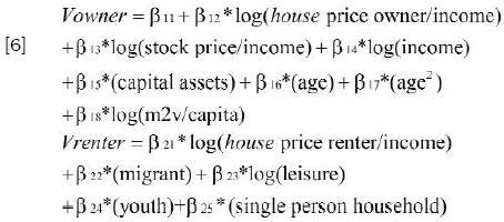
The representative utility for both forms of tenure are depicted in equation(6). It can be seen that the property sector option is a function of the owner–occupied housing flow price to income ratio, the stock price to income ratio, the property of capital assets by the households, the age of the head of the household and the average space proportionate by the dwelling. Thus, this specification presents different interrelations between monetary magnitudes such as: income, flow and stock prices. The income variable appears in various forms in the equations: first, it appears interacting with the stock price and the housing expenditure of owners and renters, this sort of formulation allows the modelling of non–random taste variation such as those originated from the fact the richer households are lesser affected by affordability issues than poorer ones; second, income appears alone in the representative utility of the property sector, this is intended to track the effects on demand of financial institutions requirements with regard to liquidity of the mortgage borrower.

Moving now to the rental sector, besides the housing price to income ratio, it appears as explanatory variables the migration status of the household (if it has moved or not from other province in the last five years), the proportion of income expended with leisure activities, the qualification of households with a head younger than 40 years old and who has not inherited a house as a gift from their parents and, finally, one variable to track if the household is composed by a single member younger than 65 years old who has not received a house as a heritage as well.

3.4. The logit model

Equation(7) depicts the logit probabilities as a function of both representative utilities introduced in equation(6):

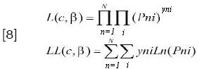
The rental sector probabilities can be generated by replacing the respective numerator in the above expression. For purposes of estimation of parameters, equation (7) can be used in the following way: A(Pni)^yni, where yni=1 if the decision maker chooses alternative i and it is 0 otherwise. So, this expression just represents the probability of the chosen alternative. If the researcher has the possibility to work with a exogenous sample, one that is collected based on factors exogenous to the choice being analyzed, then each household/individual can be treated independently from others households/individuals, the likelihood and log–likelihood function of this choice situation becomes:

 

4. Empirical results

4.1. Geographic differences and the scale parameter

In the estimations below, it will be used differing geographical regions in the analysis, such as large, medium and small cities, that can hypothetically differ in their overall scale of error variance. This fact is important, since the level of variance is intrinsically related to the level of utility. In other words, setting the level of the variance automatically sets the value of the utility: if Unj=Vnj + ε is multiplied by λ then U^*nj=λVnj + λg and the variance of the new error term, ε*=λg, becomes Var(λε)=λ²Var(ε).

If the variance of the unobserved factors differs by a significant amount, among different regions, the estimated coefficients have to be corrected in order to make the results comparable. For instance, the model for large and small cities becomes:

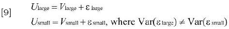
An equivalent model can be generated in which both variances assume the same value. This can be achieved by normalizing the scale of one of the equations and dividing the other by the square root of the ratio of variances α= Var (εsmall)/Var (ε large):

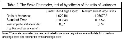
Therefore, the division of one of the equations by the square root of the ratio of variances causes the equality of the variance of the whole data set. The parameter can be estimated along with other parameters of the representative utility by maximum likelihood procedures. In the Spanish case, the scale parameter for large, medium and small cities is depicted in table 2. The ratios are very close to one, meaning that the original estimated results are a good representation of the true parameters.

4.2. The level of probabilities and elasticities

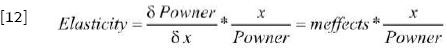
In order to properly measure the marginal effect of the explanatory variables over probabilities, it has been calculated the partial derivative of the logit probability in relation to the explanatory variables of the two tenure choice equations:

If representative utility is linear in the explanatory variable with coefficient β then the above marginal effect becomes βx(Powner*Prenter). Otherwise, if the explanatory variable in the representative utility is log transformed then the derivative assumes the form (Powner*Prenter). It is interesting to notice that these derivatives are bigger when the probabilities are closer to 0.5. In other terms, the derivative is larger when the doubt about the choice is greater. This fact produces important consequences to the Spanish case in which the estimated probabilities of being an owner, for the national data set, is very high, 85.42% in relation to the probability of being a renter 14.57%. This trend is aggravated when the size of the cities are smaller since the tenure choice division becomes more extreme as the city gets smaller, as can be seen in table 3. The probabilities have been measured using the method of sample enumeration in which the individual choice probabilities of each observation are averaged over decision makers. The weight represents the reciprocal of the probability that the decision maker was selected into the sample.

The results to be depicted in the subsequent sections, the estimated parameters and the elasticities, are influenced by this property of the logit functions. Since the marginal impacts are a function of the level of probabilities and the elasticities are function of marginal effects these last aggregated measures are impacted as well by the level of the probabilities

4.3. Stylized facts

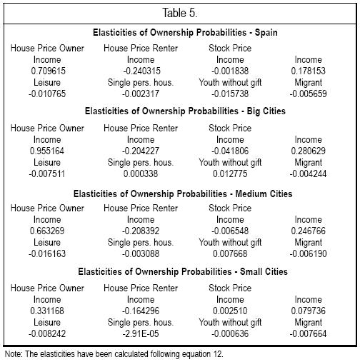
The first striking feature, about the parameter estimations in table 4 and elasticities in table 5, is the confirmation of the broad stylized facts about tenure choice already found in other works in the literature: that the incidence of homeownership rises with the age of the head of the household at a decelerated rate and that the homeownership rate rises with the level of permanent income. The trend about the age variable can be checked in table 4 by noticing that the parameter for the linear term is positive and for the quadratic term is negative. In terms of the income variable it is more interesting to look at the elasticities in table 5 where it can be confirmed that as the income variable increases the ownership rate is positively impacted in all geographical sets analyzed.

Another evidence found is that the housing flow price to income ratio provoke disproportional impacts for owned and rented dwellings. In other words, as cited by (Fallis, 1985, pp. 37–42), the relative price of housing services under different tenure does affect the choice.

4.4 Flow prices, stock prices and income

Looking at the elasticities of the ownership probability, in relation to the monetary variables, the first striking feature is the relative stronger impact of the housing flow prices to income ratio in the homeownership rate: the impact is two to four times larger in magnitude than those found for the rented houses. These figures suggest that as households become more indebted, in terms of housing expenditures, they prefer to consume housing services as owners. This interpretation is corroborated by the marginal impact of the proportion of expenditure in leisure activities: the increment in this latter variable provokes a decreasing in the probability of being an owner. More intuitively, households that have a great preference for spending in leisure activities also have a greater preference for consuming housing services as a renter. This may happen because renters do not need to save large proportions of their income in order to face the required down payments and closing costs needed in the consumption of owned dwellings. Nevertheless, as the housing expenditure increases, less is available for leisure and part of the incentive to hold a house as a renter is missed.

Another important factor for financial institutions is the capacity of households to raise the resources needed to pay the down payment and closing costs of the mortgage loan. These costs are a function of the stock price of the house, usually a percentage ranging from 15 to 40% of the total value. In terms of estimation results, the stock price, at the national level, behaves as expected being a factor that creates a barrier in the consumption of housing services through the property sector market. This effect, though, is not so severe as can be checked by the small marginal effect found for this variable, the parameter in the logit equation, for the national data set, is not significantly distinct from zero. The impact of the stock price seems to be stronger as the price increases over some threshold, see the analysis for the housing market of big cities.

4.5. The rental sector–migration, young heads and single person families demand

The mobility of persons between regions of the country is one of the main factors to explain the preference of some housing consumers for renting dwellings. As commented before, this preference is associated with the lower transaction costs that face renters in relation to owners. This stylized fact, is corroborated by the estimations above, in which the fact of having migrated from other provinces in the last five years produces a positive marginal effect in the probability of renting for all the different regions studied.

Another factor that impulses the demand for renting dwellings seems to be related to the purchase power of the households: therefore, being the head of the household a young person that has not received a house as an inheritance or being a single person family enhances the probability of being a renter.

4.6. The housing market in big cities

The first remarkable feature of the housing market in big cities is the stronger level of probability elasticities in relation to other geographical divisions. As commented before, this is in part due to the more even tenure choice distribution found in large cities, the estimated probabilities, presented in table 3, are 0.807526 for the property sector and 0.192474 for the rental sector.

Other relevant characteristic is the stronger relative impact of the housing flow price to income ratio found for owned occupied dwellings in relation to the rental market: this ratio has a magnitude of 4,68 much bigger than the one found in the remaining regions. This fact indicates a tendency for more indebted households to become owners in big cities. The behaviour of the parameters used to measure the influence of young heads and the single member family corroborate the assertive: both are positive for this geographical subdivision, meaning that even these segments, that suffer relative more from affordability problems, have a greater tendency to search for property dwellings.

Another distinctive feature of the referred market is the importance of the stock price as an inhibitor factor in the demand for ownership. In no other geographical sub–division this factor is so relevant: the elasticity in relation to the number of years required to buy a house is of –0.041806, a magnitude much higher than those found in other regions. The impact of the stock price is lower than the impact of housing flow prices because financial institutions have mechanisms, such as the enlargement of terms of payment and the reduction of down payments, to alleviate the amount of repayment required each month for the amortization of the mortgage loan. However, if the increase in the stock price is very strong even those mechanisms could not be sufficient to alleviate the requirements of savings to buy a house.

4.7. The housing market in medium cities

In medium cities, the impact of the housing flow price to income ratio for owned occupied houses in relation to the rental sector is much weaker than in big cities. The ratio reaches the magnitude of only 3.18. This find suggests that relative flow prices are less important for this region sub–division. The pattern followed by the leisure variable also helps to explain this trend. In medium cities, the probability elasticity in relation to the leisure share in total consumption is stronger than the elasticity found in big cities and in the whole country.

A peculiar feature of medium city market is the weaker importance of the stock prices in the demand for ownership. Its impact is much smaller than the one found in big cities. This may indicates that the smaller the cities are, the less valuated is the urban soil and, therefore, houses are cheaper causing less impact on the demand for property dwellings.

A final remark refers to two aspects related to the rental sector: first, the effect of being a single member family in the probability elasticity of ownership is again negative oppositely to what happens in big cities; second, the impact of being a migrant from other provinces is strengthen in this sub–region.

4.8. The housing market in small cities

As expected, small city markets are characterized by the lowest impact of monetary variables over choice probabilities. In this region sub–division the impact on the housing flow price to income ratio in the property market is only 2,01 times higher than those found in the rental market. Furthermore, income has the weakest impact of all.

The stock price provokes a positive impact on the demand for property dwellings. This corroborates the urban economic theory in which land prices decreased in the border of cities as well as in less urbanized locations.

Finally, the rental sector, of this region sub–division, is the one that most resembles the pattern followed by the national data set. The four variables that most contribute to the probability of being a renter (leisure expenditures, being a single person household, being a head of a family that has not received a house in inheritance and being a migrant from other province of the country) have all their proper sign.

 

5. Conclusions

The work confirmed, in the Spanish case, the broad stylized facts about tenure choice: that the homeownership increases with income and age of the head of households. Also, it was found support to the importance of relative prices in the tenure choice decision as defended by the neoclassical theory. These results are robust on different data sets for the various city sizes studied in this work.

The work stressed the relevance of affordability indicators in the determination of economical preferences of households. Thus, the role of monetary variables in the determination of the housing tenure choice was object of intense research. The mentioned variables entered the discrete choice model in an interactive way: for instance, it was employed the housing flow price to income ratio and the stock price to income ratio as explanatory variables. The stock price behaved as a homeownership inhibitor is large cities in which its values started to become excessively high.

An important result of the work was the finding of a positive correlation between leisure expenditures and household's preferences of being a renter. This fact is corroborated by economic theory that in principle considers possible that some households may find lifetime utility higher as a renter than as an owner. The election of being a renter implicitly means a given pattern of expenditure and saving during the whole life of the consumer.

Another concern of the study was the differences between parameter estimates in cities with three distinct populations: lower than 10.000 inhabitants, between 10.000 and 50.000 and more than 50.000. The results have shed light on important dissimilarities that may produce great impacts in terms of policy actions in the sector. For instance, the impact of relative prices in tenure choice decisions are significant distinct among different city sizes. This is a very important result since the magnitude of the parameters used to track the effect of relative price in the logit equation is considerably bigger than the remaining parameters. Moreover, the impact of variables such as the youth of the head of the household, which has not inherited a house, over the probability of home–ownership increases as the city gets smaller. This latter phenomenon also happens with the migrant status of the households, as the city gets smaller the positive impact on the probability of being a renter increases.

The comparative results among cities of distinct sizes have to be analyzed with caution. Aggregated results, such as marginal effects and elasticities, are functions of the current level of probability choices. This fact has a great importance in the Spanish case in which the market shares of the rental and property sector are very extreme. The major part of discrete choice models, including logit models, have a sigmoid shape that give more relevance to changes in representative utility of consumers experiencing a greater level of uncertainty in their choice. Thus, since in the Spanish case there is a considerable preference for homeownership, it is more difficult to implement politics to foster the demand of housing in the rental sector.

A final remark is that the work found a variable pattern in the probability of choosing a determined tenure status for differing sort of households. The young heads and the single member family groups seemed to behave differently depending on their share of housing expenditures in their total budgets and the size of the city in which they were living. These groups are more willing to be owners as the city gets larger and to engage into the rental market in the opposite situation. Many politicians defend the focus in these segments when designing housing policies without paying attention to the aforementioned differences in preferences. This can cause serious problems of non–participation in government programs.

 

Data appendix: variables employed in the tenure choice equations

The original source of all the data employed is the "Encuesta de Presupuestos Familiares – 90/91, the main Spanish Household Survey.

HOUSE PRICE OWNER – represents the flow housing price paid periodically in the property market. The measure has been corrected by hedonic price procedures.

HOUSE PRICE RENTER – Is the flow housing price paid periodically in the rental market. The measure has also been corrected by hedonic price procedures.

STOCK PRICE – This series was generated with data from the Ministry of Development (Ministerio del Fomento): this public organism publishes a quarter series of the square meter housing stock prices for various city and regions of the country. In order to generate the final series, it has been multiplied the square meter prices by the dimension of the dwelling, also depicted in square meters, present in the EPF (90–91).

INCOME – Is the permanent income measure calculated as mentioned in the text.

CAPITAL ASSETS – Is a binary variable that reflects whether the household holds financial assets or not: (1) if it does; (0) if it does not.

AGE – Is the age of the head of the household.

M2/MEMBERS – Represents the division of the square meter size of the dwelling by the number of household members.

EXPENDITURES IN LEISURE ACTIVITIES – Represents the share of total expenditure spend in leisure activities.

YOUTH WITHOUT INHERITANCE – Is a dummy variable that represents if the head of the household has less than 40 years and at the same time has not inherited a house. single person household – A dummy variable for the kind of household: (1)

SINGLE PERSON HOUSEHOLD with the head with less than 65 years old; (0) other households.

 

References

Borsch–Supan, A. (1987) Econometric Analysis of Discrete Choice With Applications on the Demand for Housing in the U.S. and West Germany, Lecture Notes in Economics and Mathematical Systems, Springer–Verlag, Managing Editors: M. Beckman and W. Krelle, pp. 105–115.        [ Links ]

Bover, O. and Velilla, P. (2001) Precios hedónicos de la vivienda sin características: el caso de las promociones de vivienda nuevas, Bank of Spain, Servicio de Estudios Económicos, n° 73.        [ Links ]

Deaton, A. and Muellbauer, J (1991) Economics and Consumer Behaviour, Cambridge University Press, pp. 97–108.        [ Links ]

Dispaquale, D. and Wheaton, W. C. (1996) Urban Economics and Real State Markets, Prenctice Hall, pp. 186–188.        [ Links ]

Dulce Tello, R.M. (1995) "Un modelo de elección de tenencia de vivienda para España", Moneda y Crédito, 201, pp. 127–152.        [ Links ]

Fallis, G. (1985) Housing Economics, Butterworths Toronto, pp. 37–42.        [ Links ]

Gonzáles Páramo, J.M. and Onrubia, J. (1992) "El gasto público en vivienda en España, Hacienda Pública Española, n° 120/121, pp. 189–231.        [ Links ]

Herderson, J.V. and Ionnides, V.M. (1983) "A Model of Housing Tenure Choice", American Economic Review, 73 (1), pp – 98–113.        [ Links ]

Mayer, C.J. and Engelhardt, G.V. (1996) "Gifts, Down Payments, and Housing Affordability, Journal of Housing Research. Vol. 7(1), pp. 59–77.        [ Links ]

McFadden, D. (1978) "Modelling the Choice of Residential Location", in A. Karlquist, L. Lundquist, F. Snickars and J. Weibull, Spatial Interaction Theory and Planning Methods, pp. 75–96.        [ Links ]

Olsen, E.O. (1986) "The Demand and Supply of Housing Service: A Critical Survey of the Empirical Literature", in: Handbook of Regional and Urban Economics, Volume II, Chapter 25, Edited by E.S. Mills, pp. 989–1022.        [ Links ]

Train, K.E. (2001) Discrete Choice Methods with Simulation, Cambridge University Press.        [ Links ]