nova página do texto(beta)
 Inglês (pdf)
 Artigo em XML
 Referências do artigo
 Enviar este artigo por email
 Citado por SciELO
  Similares em
SciELO
Similares em
SciELO 
 Permalink
Introduccion
The Efficient Market Hypothesis (EMH) (Fama, 1970, 1991) has important implications for understanding the mechanisms that determine the performance of stock portfolios. According to the EMH, no investor can consistently earn abnormal returns using currently available public information without undertaking additional risk. There are numerous empirical studies that test the EMH, and the results of a vast majority support the conclusion that the pricing mechanism at work in modern capital markets is a “fair game”, i.e., markets are highly efficient in reacting to the arrival of new information, and that risk and return are highly positively correlated through long periods. While EMH opponents point out frequent evidence of under- and over-reaction episodes in securities markets, no conclusive rejection of the EMH exists. In any case, the EMH is the best-known description of financial securities’ price movements. If an analysis departs from the assumption that markets are efficient, investors can estimate the expected returns of individual securities using one or several well-known equilibrium models (such as CAPM, APT, among others), according to which returns are primarily a function of risk (total risk and systematic risk). With the expected return as a discount rate, the price of a security reflects the present value of its expected future cash flows. However, the estimation of the present value of those cash flows must incorporate a variety of risk factors, such as volatility, liquidity and bankruptcy. Portfolio diversification reduces the weighted average of the individual portfolio securities’ variance of returns, as long as they are less than perfectly positively correlated. However, diversification only dilutes the unsystematic risk component, i.e., systematic risk cannot be eliminated through diversification. The most relevant implication is that there is a limit beyond which diversification can no longer reduce portfolio return risk.
The abandonment in 1973 of the Bretton Woods Agreement that unchained all countries’ currency exchange rates from fixed parities with respect to the U.S. dollar, allowing them to be henceforth determined by market forces, resulted in increasing market volatility not only in the exchange rates themselves, but also the prices in different commodity markets (oil, copper, etc.), thus creating the urgent need for hedging mechanisms for many types of economic agents. Modern financial markets responded swiftly, creating and making available to market participants a variety of financial contracts that help investors reduce their exposure to market risks. Nowadays, futures, forwards, swaps and options contracts on a wide diversity of underlying assets are available to deal with market risk in a disciplined and orderly fashion. The proliferation of derivative contracts on stock indices responded to the high costs associated to modifying the composition of widely diversified portfolios as market expectations about the future change. Some of these contracts convey the right and the obligation to buy or sell a given position in financial securities, commodities, currency or several other categories of underlying assets, and their effective cost is low (such as futures contracts, where the “round-trip” fee is around $15 US). Others convey the right, but not the obligation, to buy or sell, and the holder can decide when it is convenient to exercise the contract, albeit at a higher cost.
Following Koulis et al. (2018), the intense volatility and complexity of financial markets have made the optimal hedge ratio (the optimal number of future contracts that an investor must include in his/her portfolio to obtain the most effective protection from adverse market movements) a subject of the highest consideration for practitioners and academia. The objective of this study is to contribute to that line of research by examining the case of the future contract (IPCF) of the Mexican Stock Market index (IPC). The hypothesis postulated is that to design and implement an effective hedging strategy it is important to consider the volatility of the time series, underlying asset and futures contract as time-varying. Testing consisted of critically discussing different hedging strategies based on the Mexican Stock Market Index Futures contracts for a period from December 30th, 1999, through December 30th, 2016. The hedging strategies included in this experiment are: a) a No-Hedge strategy; b) a Naive Hedge Ratio Strategy; c) a Constant-Hedge Strategy (obtained using an OLS regression with a HAC Newey Covariance Matrix); and d) a Dynamic Hedge Strategy, based on a Constant Conditional Correlation Multivariate GARCH model with asymmetric variations. Finally, we compare and evaluate the above strategies using different risk measures to verify how closely the ex-post performance of each hedging strategy corresponds to the ex-ante investor risk tolerance choice. Our results suggest that the Asymmetric Constant Conditional Correlation M-GARCH (Asymmetric CCC) model (which recognizes the possibility of different responses in volatility depending on whether innovations are positive or negative) eliminates risk more efficiently than the No-Hedge or the Constant-Hedge strategies. The Asymmetric CCC proves to be the best choice from the point of view of ex-post performance in terms of correspondence with ex-ante risk tolerance choice. However, in terms of portfolio returns only, our results indicate that No-Hedge is the best performing strategy (consistent with the well-known trade-off theory between risk and return). The following section presents a sample of the most influential works in the literature on risk hedging. The third section introduces the data and the methodology used in the empirical section. The fourth section present the results of the estimations and their interpretation and, finally, the fifth section concludes.
I. Literature review
The modeling of the second moment of financial asset return distributions has been a major field of study over the past few decades. Since Mandelbrot’s (1963) seminal work, there has been a generalized interest in exploring volatility models, most notably pioneered by Engle (1982) and Bollerslev (1986). Volatility models have developed in many ways - univariate for individual assets and multivariate for combinations of asset portfolios. Research has focused mostly on such aspects as the in-sample volatility of models, using diverse specifications, but fewer studies have addressed the out-of-sample robustness of these models, even when they, at least conceptually, could be of greater importance for practical applications among portfolio managers, risk managers, etc. Different authors postulate that a better understanding of the distribution of commodity cash and futures contracts’ prices is crucial to estimate optimal hedging strategies. For example, Baillie and Myers (1991) examined the daily price data of six different commodities over two futures contract periods and modeled individual commodity price movements using the GARCH framework. According to these authors, the specification advantage of the latter is that “very convenient assumptions about the conditional density of commodity price changes, such as the normal or t distributions, can lead to a rich model that allows for time-dependent conditional variances and leptokurtosis in the unconditional distribution of price changes.” Arguably, GARCH models had already proved to be useful in explaining the distribution of common stock prices, so these authors show that they are equally effective in describing the distributions of commodity cash and futures prices, and that they lead to a natural description of time-varying optimal hedge ratios in commodity futures markets. This latter strategy is implemented using bivariate GARCH models to compute the conditional variances under three alternative portfolio strategies: a) no hedging; b) hedging with a constant Optimal Hedge Ratio (OHR) estimated using a simple Ordinary Least Squares (OLS) regression; and c) hedging with a time-varying OHR. Some simple performance tests indicate that the usual assumption of a constant hedge ratio is quite costly in terms of a higher return variance for some commodities (coffee, corn and cotton), but not for others (beef, gold, and soybeans).
The inclusion of Multivariate Generalized Autoregressive Conditional Heteroskedastic (M-GARCH) models in the most frequently used econometric software packages represented a major step forward and gave an important impulse to time series volatility modeling. The most important and distinctive feature of M-GARCH models is their flexibility in incorporating time-varying conditional covariances and variances. Both can be of substantial practical use for modeling and forecasting the volatility of many diverse assets such as stocks, bonds, commodities, exchange rates, etc. But, among the many interesting applications of M-GARCH models in the field of finance and investments, these models represent a major improvement in the calculation of time-varying hedge ratios using futures contracts, including the possibility of discriminating the volatility response to an innovation depending on whether it is positive or negative in sign (Brooks et al. 2002; Brooks and Persand, 2003).
The most conventional method for estimating optimal hedge ratios is to use the slope coefficient from a simple OLS regression of spot prices on futures prices, where the slope coefficient reflects the ratio of the unconditional covariance to the unconditional variance of the futures prices. However, instead of applying a regression model, the OHR can be obtained from the second moments of the joint distributions of spot and futures prices. Lien and Luo (1994), for example, argue that the advantage of the Conditional Heteroskedasticity Models (ARCH and GARCH) is that conventional conditional density assumptions allow for time- dependent conditional variances and leptokurtosis in the unconditional distribution, and propose a breakthrough innovation. While most previous studies contemplate only one-period hedging decisions, they consider that “realism suggests that the representative hedger`s planning horizon covers multiple periods.”
Recognition that covariance matrix forecasts of financial asset returns are an important component of current practice in financial risk management led Lopez and Walter (2001) to evaluate the relative performance of different covariance matrix forecasts using standard statistical loss functions and a Valueat-Risk (VaR) framework. In their work, these authors postulate that, given the wide variety of volatility models, the key question is how best to choose among them. They examine VaR estimates obtained from a wide variety of multivariate volatility models, ranging from naive averages to standard time-series models and option contracts-implied volatility models. Their evaluation is based purely on out-of-sample covariance matrix forecasts and employs both statistical loss functions and a VaR framework that represents an innovation with respect to previous studies. They find that models generated from option prices in foreign-exchange portfolios perform best under statistical loss functions, and that within a VaR framework the relative performance of covariance matrix forecasts depends greatly on the VaR models’ distributional assumptions.
Brooks et al. (2002) introduced a method for evaluating alternative OHR strategies in a modern risk management framework, highlighting the importance of allowing OHR to be time varying, and innovate by introducing the possibility of volatility responses behaving in an asymmetric fashion. At the time they published their study, the general consensus was already that the use of MGARCH models resulted in superior performance portfolios as measured by return volatility, relative to either time-invariant or rolling ordinary least squares (OLS) hedges. These authors’ original contribution consisted of linking the concept of optimal hedge ratios with the notion of News Impact Surface (Kroner and Ng, 1998) and recognizing that if the hedging surface of the OLS is determined independently of the news that is constantly arriving in the market, it could produce suboptimal results. To incorporate new information into a dynamic hedging strategy, they propose considering the impact of asymmetry on time-varying hedges that use financial futures. The assumption is that an asymmetric model that allows conditional volatility forecasts of cash and futures returns to respond differently to positive and negative return innovations should produce superior hedging performance. Additionally, they show how the effectiveness of hedges thus obtained can be evaluated by calculating the minimum capital risk requirements (MCRR), adapting a method developed by Hsieh (1993). The most important findings reported by Brooks et al. (2002) are that any type of hedge, even a naive hedge, is better than a “naked” position and that, at short investment horizons, there are large gains to be made by allowing the hedge to vary over time.
More recently, Park and Jei (2010) propose extensions of Bollerslev’s (1990) Constant Conditional Correlation (CCC) and Engle’s (2002) Dynamic Conditional Correlation (DCC) models to introduce two more flexible models to analyze the performance of optimal conditional hedge ratios. They propose a) adopting bivariate density functions, such as a bivariate skewed-t density function; b) using asymmetric individual conditional variance equations; and c) incorporating asymmetry in the conditional correlation equation for the DCC-based model. They also conduct a portfolio performance evaluation in terms of variance reduction, Value at Risk and Expected Shortfall. To define the specification of the conditional mean of their M-GARCH models, they recognize that there are shortrun deviations from the stable long-run relationship which may be due to the temporary disequilibrium of either the spot or the futures markets, transaction costs and other microstructure conditions. For that reason, after confirming the presence of cointegration among the series, and following previous studies (e.g., Brooks et al. 2002; Lien and Yang 2008), Park and Jei (2010) use a VECM specification for the conditional mean equation of their model.
In the same line as Brooks and Persand (2003), Lien (2005) contributes to the theoretical analysis of the asymmetric impact of innovations on volatility and, thus, on futures hedging. However, considering the GARCH framework as not analytically tractable, this author chooses the stochastic volatility model, a close substitute. Lien’s work extends his own previous study (Lien and Tse, 1999) from a symmetric stochastic volatility model to an asymmetric model. His modeling strategy considers building an asymmetric approach that allows different volatility responses to good and bad news and finds that the average optimal hedge ratio increases as the degree of asymmetry-in-response increases. Notwithstanding, the hedging performance remains unchanged.
The hedging effectiveness of hedge ratio building models, like most fields in the discipline, progressively incorporates more realistic characteristics. For example, Sheu and Lee (2014) argue that the rationale for using dynamic hedge ratios is that the spot price and futures price series are more adequately described as time changing distributions. So, to estimate a Minimum Variance Hedge Ratio one needs to estimate the conditional variance of both spot and futures return series. However, while frequently used multivariate GARCH models are capable of capturing the time-varying covariance structure of spot and futures returns, they do not take into account regime-shifts due to changing market conditions. To address this problem, they propose the use of a Multichain Markov Regime Switching GARCH (MCSG) model that allows the changing dynamics of spot and futures returns series to be governed by different state variables and apply it to futures contracts of platinum, palladium gold, silver, and heating oil traded in the New York Mercantile Exchange (NYMEX), corn and wheat futures contracts traded in the Chicago Board of Trade (CBOT), and cocoa and sugar traded in the New York Board of Trade (NYBOT) between January 1991 and December 2010. The empirical results reported by this study reveal that the MCSG strategy exhibits a superior hedging performance compared to the Constant Correlation GARCH model, which assumes a constant regime correlation. When compared with three single-state, variable-dependent time-varying correlation GARCH models in-sample performance, MCSG proves the best evaluated for corn, heating oil, palladium, platinum, and gold. Furthermore, the out-of-sample performance of MCSG is always better than the CC for all commodities. The closing conclusion of this work is that the superior hedging effectiveness of the strategies that contemplate a nonzero cross-regime probability confirm the importance of modeling spot and futures returns with the multichain regime switching model. Billio et al. (2018) develop a new Bayesian multi-chain Markov-switching GARCH model for dynamic hedging in energy futures markets which, they argue, has important consequences for portfolio risk management and energy trading. The model identifies the different states of discrete processes as volatility regimes and uses regime-switching models with multiple correlated chains, which are more flexible than single-chain models. based on which it is possible to define a “robust minimum variance hedging strategy”. When the strategy is empirically tested with oil spot and futures markets, the authors report strong evidence in favor of their methodology when contrasted with alternative models. Another good example of recent studies that uses sophisticated hedging strategies is the work of Chang et al. (2011), who compare five different volatility modeling strategies (CCC, VARMA-GARCH, DCC, BEKK and diagonal BEKK) to hedge the exposure to WTI and Brent crude oil price fluctuations. These authors’ analysis finds that the optimal hedge ratios for Brent should be holding futures in larger proportions than spot, but, in the case of the WTI market, the DCC, BEKK, and diagonal BEKK models suggest holding crude oil futures to spot. Moreover, when the CCC and VARMA-GARCH are considered, they conclude the best strategy is holding crude oil spot to spot. In terms of the hedging performance of the different strategies, the paper concludes that diagonal BEKK is the best and BEKK the worst for calculating an optimal hedge ratio with the objective of reducing portfolio risk.
For a recent complex study that combines different estimation techniques with time-series analysis and data from emerging markets, the paper by Singh et al. (2019) is a good example. They examine the hedging performance of two emerging markets’ equities indices (Morgan Stanley Capital International -MSCIEmerging Market -EM- and MSCI-BRIC -Brazil, Russia, India, and China) with two globally traded commodities indices (Standard & Poor’s Goldman Sachs Commodity Index - GSCI- and Bloomberg Commodity Index -BCOM), and two financial factors (the implied volatility index of S&P 500 index -VIX- and the US bond futures-BOND), using daily data from January 4, 2004 through November 30, 2017. The authors present an analysis that first examines the wavelet coherence among these indices, then perform a connectedness analysis, and, finally, estimate the dynamic conditional correlations models to calculate time-varying hedge ratios and use rolling-windows to estimate one-step-ahead forecasts of dynamic conditional volatility. The results reported find “the existence of a higher level of dynamic coherence and connectedness between equities and commodities benchmarks”, which implies that decision makers do not really care much about the integration of these indices. The extent of co-movement is also very high for the pair of EM and BRIC. Interestingly, the paper reports that both emerging market indices (EM & BRIC) have a negative correlation with VIX and BOND. The most surprising finding is that the VIX is the most desirable asset for hedging choices, followed by BCOM and GSCI, meaning that the emerging markets equities indices may combine with commodities indices “for hedging and risk diversification purposes.”
A representative example of the increasing robustness of testing approaches followed by studies interested in learning more about the optimal hedge ratio determination and some eye opening results, is the paper by Wang et al. (2015), where the authors compare the hedging performance in twenty-four futures markets of minimum-variance hedging strategies whose underlying assets include commodities, currencies, and stock indices, based on the covariance parameters from eighteen econometric models. They compare their performance to the naive hedging strategy and determine that it is difficult to find a minimum variance strategy that consistently outperforms the simple naive strategy before transaction costs. These authors also report that if the transactions costs are considered, those strategies with time-varying hedge ratios (requiring frequent rebalancing of the hedge ratio) perform even worse than the naive hedging strategy, something that should be obvious considering that the latter incurs only the initial and terminal transaction cost. Their robustness tests include repeating the analysis for different observation periods, hedging horizons and out-of-sample, to find that the naive hedging strategy consistently performs as well as other strategies. They conclude their work by expressing their belief that estimation errors and model misspecification may probably explain the results they report.
In the context of Latin America, the liberalization of important economic sectors has created new financial need to support their daily operation, as in the case of Colombia where the development of the wholesale energy market originated a growing negotiating of electricity futures contracts in the local capital market. The work of Diaz-Contreras et al. (2014) describes the favorable conditions that economic development of the energy industry has created for the development of new financial contracts to hedge the exposure of both producers and consumers of electricity, one of which has been precisely the futures contract, and propose the development of an option contract whose underlying asset is the same commodity. More specifically, they propose the design of an exotic option barrier-type contract on electricity. Modelling intraday volatility in the price of electricity in Colombia, the authors found high volatility and explain it by the past behavior of the spot and futures price of electricity. Using Value at Risk (VaR), the authors estimate the maximum loss faced by a typical agent in the electricity market and confirm the need for hedging instruments. However, this paper concludes that one of its main limitations is that the contract they develop is only conceptual since, at present, there are no publicly traded options on electricity in the Colombian market, so they consider their proposal should be incorporated to contribute to a more transparent and efficient mechanism of price formation. In the case of Mexico, De Jesus (2016) studies dynamic efficient cross-hedging strategies for the country’s oil market. Extending Engle’s (2002) and Tse and Tsui’s (2002) Dynamic Conditional Correlation models, this author incorporates an error correction term in the equations of the conditional mean to develop optimal minimum variance cross-hedging strategies for the three varieties of Mexican crude oil (Olmeca, Istmo, and Maya) prices. According to the out-of-sample results reported in this paper, the cross-coverage strategies, based on the MGARCH-DCC improved with a correction term in the conditional mean equation model, reduce an oil producer/consumer’s exposure when using WTI and Brent futures contracts by as much as 77.91 percent and 98.95 percent, respectively, for Olmeca crude; 75.09 percent and 71.62 percent, for Istmo; and 64.48 percent and 68.07 percent for the Maya crude oil varieties. In comparison, the maximum effectiveness of the OLS model in terms of risk reduction in the case of the Olmeca crude oil variety is 62.11 percent and 50.42 percent, respectively (always with reference to the WTI and Brent futures contracts).
There is an abundant literature that studies stock market indices’ hedging strategies using many different methodologies and contemplates a wide variety of countries, making it a challenge to cover them reasonably well in a short literature review, such as the one we seek to introduce in this section. Therefore, we only briefly discuss some illustrative cases in the following lines. Brooks and Persand (2003) compare the performance of various GARCH models, “some of which do, and some of which do not, allow for asymmetries”. Their study focuses on the stock markets of five Southeast Asian economies and utilizes the S&P 500 index as a benchmark. The models proposed by these authors are contrasted within the rules of the Basle Committee and the methods proposed for the calculation of Value at Risk (VaR) are reliable, using a holdout sample. They conclude that models allowing for asymmetries can lead to an improvement in VaR estimates. Chohudry (2004) investigates the hedging effectiveness of large Pacific Basin stock market futures contracts (Australian, Hong Kong, and Japanese stock futures contracts), using weekly returns from January 1990 to December 2000. He compares the naive (one-to-one) hedge ratio with the minimum variance hedge ratio (both are constant) and the GARCH model hedge ratio (which is time-varying). The effectiveness of each strategy is evaluated by comparing two 1-year, out-of-sample periods. Using the performance of the three ratios, the author concludes that the time-varying GARCH hedge ratio almost always outperforms the constant ratios. The only exception is the case of Hong Kong where the GARCH time-varying hedge underperforms both of the constant hedge ratios. While the reported evidence is clearly in favor of time-varying hedges, the author leaves open the choice between constant and time-varying hedge ratios by suggesting that the trade-off between risk reduction and transaction costs of the GARCH hedging method is what must be considered by the practitioner. Lee et al. (2009) use data from for six stock markets (Korea, Singapore, Japan, Taiwan, Hong Kong and the United States), combined with the Taiwan Stock Index Futures, S&P 500 Stock Index Futures, Nikkei 225 Stock Index Futures, Hang Seng Index Futures, Singapore Straits Times Index Futures, and Korean KOSPI 200 Index Futures, to examine four static and one dynamic hedging model (OLS, Mean-Variance Hedge Ratio, Sharpe Hedge Ratio, and MEG Hedge Ratio) with the aim of finding the optimal hedge ratio and exploring their hedging effectiveness under different investment horizons. Interestingly, they find that the best method for conducting optimal hedge ratio strategies in different markets is not the same. Hedging strategies with the S&P 500 Index Futures outperform other stock index futures when the hedge ratios are obtained using static models. In the case of the Asian markets, the Nikkei 225 Index Futures proves the most effective in Asia, with the Hang Seng Index in second place, STI in third, and the KOSPI Futures fourth. The hedging effectiveness of TAIEX Index Futures is reported as the least successful in the sample of Asian markets. Koulis et al. (2018) investigate the hedging effectiveness of Futures Markets from the United States and Europe using the S&P-500, DAX, FTSE/ATHEX-20, IBEX and PSI spot and futures daily closing prices from January 4, 2010, through December 31, 2015. Hedge ratios are calculated using three alternative econometric methods: an Ordinary Least Square Model (OLS), an Error Correction Model (ECM) and an Autoregressive Distributed Lag (ARDL) cointegration model. The results reported show that with the ARDL cointegration model, time varying hedge ratios are more efficient than the fixed hedge ratios in minimizing risk, and that this superior performance of more sophisticated econometric models is even more noticeable when applied to date from the periphery capital markets of Europe (Spain, Italy, and Greece).
II. Data and methodology
Emerging markets’ stock investments are attractive to the average investor not only because of their frequent above average returns, but also because of the diversification benefits they bring to investors’ portfolios. However, investors frequently consider disinvesting their Emerging Markets securities and converting their holdings into hard currency when they anticipate (or experience) the presence of turbulent international market conditions (e.g., the 2007-2009 Global Financial Crisis, or the more recent European Sovereign Debt Crisis) or a period of domestic economic instability due to shocks in the main commodities’ exports markets, trouble in local banking systems, currency exchange rate problems, etc. An alternative open to investors is to use hedging strategies that protect their portfolio’s value from short-term adverse environmental conditions. However, not many Emerging Markets have domestic derivatives markets where investors can find specialized contracts, so international investors find the few emerging markets where that possibility exists relatively more attractive. The case of the relatively young MexDer (created in 1998) is an example of a derivatives markets in an emerging country that has a promising future, where a variety of futures and options contracts on the local stock market index, known as the IPC, and several other securities and commodities are traded. Our interest in this work is centered on the use of the MexDer Futures contract on the IPC as a hedging instrument to implement hedging strategies for diversified portfolios that contain Mexican stocks. More specifically, we aim to identify which, among several possible hedging strategies, is the best in terms of risk reduction, and from the point of view of the portfolio’s returns. The data used consists of daily observations of the IPC, and its futures contract, from December 30th, 1999, through December 30th, 2016. In total, the sample consists of 4,282 daily observations. All the series are retrieved from a Bloomberg terminal. Bloomberg provides a time series of rolling IPC futures quotations for the next four expiration dates at any given time, and labels them IS1, IS2, IS3 and IS4, with IS1 being the nearest expiration date and IS4 the most distant in time. The futures contract price time series was built with a rolling-hedge strategy that uses only IS1 contracts, by far the largest trading-volume contracts all the time. The rollover strategy assumes that an IS1 contract is rolled over at its expiration date, to the next expiration date contract, three months ahead. For our purposes, the futures contract series IS1 is hereafter called IPCF (IPC Future). Brooks et al. (2002) follow a similar rollover strategy, but they use a contract replacement decision based on that moment when the volume of the next-maturity future contract exceeds the volume of the most recent one. We adopt a time-criterion that is more appropriate for the MexDer, since the volume of trading is still much smaller than that of the LSE, and as few as a couple of atypical trades may cause premature rollovers when basing our modeling strategy on the volume-criterion.
This experiment consists of comparing four possible strategies in response to IPC volatility: a) a simple “no-hedge” strategy; and three different, statistically based, hedging strategies. The first statistically based strategy, also considered a “benchmark” strategy, is a so called b) “naive” strategy, and consists of using one unit of the IPCF to hedge each unit of the IPC; that is, a 1:1 fixed hedge ratio throughout the period of analysis. The second strategy, commonly used by practitioners, estimates c) a fixed hedge ratio, obtained by dividing the historical covariance of the IPC and the IPCF by its historical variance; that calculation is equivalent to obtaining the slope of an Ordinary Least Squares (OLS) regression of the IPC on the IPCF. The third and most sophisticated strategy considers a d) dynamically changing hedge ratio, estimated using conditional variances and covariances of the variables, as well as their asymmetric response to positive and negative innovations. The hedge ratio for this strategy is re-estimated each day as in equation [1] below, where βt* represents the optimal hedge ratio for period t from the conditional variance of the IPCF (VarLRIPCF,t), and the conditional covariance between IPC and the IPCF (CovLRIPC,LRIPCF,t). In the OLS case, the time subscripts are dropped and a constant optimal hedge ratio (β*) is calculated from the unconditional variance and covariance, which does not account for possible asymmetry or cointegration.
The dynamic hedge ratio is calculated with a Bivariate GARCH1 model that uses a time-varying covariance matrix for the two time-series. GARCH models originated in response to the need to study and forecast the volatility of financial assets. The relevant literature includes several transcendental seminal papers, such as: Engle (1982), Bollerslev (1986), Nelson (1991), Bollerslev and Wooldridge (1992), Glosten et al. (1993), Engle and Ng (1993), Rabemananjara and Zakoian (1993), and Engle (2002). A wide variety of improvements to conditional heteroskedasticity models have recently come to light (for an excellent review of the literature, see Terasvirta, 2009).
Multivariate GARCH (M-GARCH) models are conceptually equivalent to the univariate GARCH models in the sense that both model the volatility of different series, but the former estimates the conditional variance of several series and add conditional covariance equations at the same time. As expected, their mathematical complexity is significantly greater compared to the univariate version. M-GARCH models have developed increasingly sophisticated variations that resemble the behavior of time series volatility in a more reliable way. The most popular include the VECH (Bollerslev, Engle and Wooldrige, 1988), the Diagonal Half-Vectorization (or DVECH), which is a derivation from the VECH model where the variance-covariance matrix has been restricted to a diagonal matrix (Brooks, 2014), the Constant Conditional Correlation (CCC) model of Bollerslev (1990), and the the BEKK model (Engle and Kroner, 1995).
Following Kroner and Ng (1998), we use the following notation:
Rit: the rate of return of asset I from time t-1 to time t.
μit: the expected return of asset i given all information at time t-1.
εit: the unexpected return of asset i (εit = Rit - μit).
hiit: the conditional variance of Rit given all information at time t-1.
hijt: the conditional covariance between Rit and Rjt given all information at time t-1.
Ht: the conditional covariance matrix.
The VECH model is represented as follows:
Where
The VECH model has two important estimation problems. The first one is that the number of parameters to be estimated grows very rapidly (a 20-asset model will have 630 parameters); and the second is that the model might not produce a positive definite covariance matrix (unless nonlinear inequality restrictions are imposed) (Kroner and Ng, 1998). The Diagonal Half-Vectorization (or DVECH), which is a derivation from the VECH model where the variance-covariance matrix has been restricted to a diagonal matrix, aims to overcome these hurdles in an efficient manner (for a more detailed description of this model, see Brooks, 2014).
The BEKK model proposes a solution to the covariance matrix positive definiteness problem, where the ijth covariance may be expressed as:
Where εp and εq represent unexpected shocks to series p and q.
The Constant Conditional Correlation model restricts the conditional covariance between two asset returns to be proportional to the product of the conditional standard deviation. This time, the conditional correlation coefficient of the two asset returns is time invariant. The model can be represented as follows:
The CCC model is positive definite if the correlation matrix [ϱij] is positive definite. In this case, the number of parameters is only (1/2) N2. For a portfolio of 20 assets, the number of parameters to be estimated is 270.
The three different GARCH specifications described in the above estimations were attempted, but it was not possible to obtain convergence for the BEKK model, so only a DVECH (Bollerslev, Engle, Wooldridge, 1988) model and a CCC (Bollerslev, 1990) are included. While the DVECH model retains a larger number of parameters by estimating a correlation equation, and can provide a better in-sample fit, it is also more complex to estimate and less parsimonious than the CCC model, which might have a forecasting advantage, as mentioned before.
As is the case with univariate GARCH models, the M-GARCH versions have also seen a proliferation of alternative versions that have become very popular in empirical work, in particular, the use of models where the conditional variances and/or covariances react differently to the positive or negative nature of innovations of the same magnitude (Brooks, 2014; Kroner and Ng, 1998).
III. Empirical results and interpretation
The database used in this analysis includes daily closing price observations for the Mexican Stock Exchange Market Index (IPC) and its Future contract daily closing prices (IPCF), from December 30th, 1999, through December 30th, 2016, for a total number of 4,282 daily closing price observations. All the series are downloaded from Bloomberg Financial Services. The IPC Futures contracts have quarterly maturities in March, June, September and December.
Tables 1a and 1b show the descriptive statistics for the IPC and the IPCF, as well as for their logarithmic returns. Both series show a negative skewness in levels and a positive skewness in returns. Also, in both series there is positive kurtosis, a typical characteristic of financial returns. Such evidence also confirms that the distribution of the variables does not conform to a normal distribution according to the Jarque-Bera test. As expected, there is a very high correlation between the IPC and the IPCF, both in levels and in returns.
Table 1a Descriptive Statistics of the IPC and the IPCF.
| IPC | IPCF | |
|---|---|---|
| Mean | 25,668.70 | 25,768.97 |
| Median | 28,459.33 | 28,614.50 |
| Maximum | 48,694.90 | 48,812.00 |
| Minimum | 5,081.92 | 5,090.00 |
| Std. Dev. | 14,493.73 | 14,484.21 |
| Skewness | -0.0910 | -0.0957 |
| Kurtosis | 1.4839 | 1.4826 |
| Jarque-Bera | 416.02 | 417.31 |
| Probability | 0.0000 | 0.0000 |
| Observations | 4282 | 4282 |
| Correlation | IPC | IPCF |
| IPC | 1.00000 | 0.99997 |
| IPCF | 0.99997 | 1.00000 |
Table 1b Descriptive Stats of LRIPC and LRIPCF (log-returns).
| LRIPC | LRIPCF | |
|---|---|---|
| Mean | 0.00043 | 0.00042 |
| Median | 0.00077 | 0.00069 |
| Maximum | 0.1044 | 0.1095 |
| Minimum | -0.0827 | -0.0803 |
| Std. Dev. | 0.0132 | 0.0136 |
| Skewness | 0.0225 | 0.0432 |
| Kurtosis | 8.1215 | 8.3125 |
| Jarque-Bera | 4,679.06 | 5,035.59 |
| Probability | 0.0000 | 0.0000 |
| Observations | 4281 | 4281 |
| Correlation | LRIPC | LRIPCF |
| LRIPC | 1.00000 | 0.96973 |
| LRIPCF | 0.96973 | 1.00000 |
Source: Authors’ own, with data retrieved from Bloomberg.
Figure 1 is a graphical representation of the original series and their logarithmic returns, and confirms their highly-similar behavior in time, reaching levels of correlation close to 1 in the case of logarithms, and marginally superior to 0.9697 in the case of the log-returns.
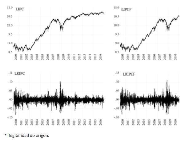
Source: Authors’ own, with data retrieved from Bloomberg.
Figure 1 IPC and IPCF logs and log-returns.
Before proceeding to test if the series are stationary, a brief digression is required. During the sample period, different events had a strong impact on the stability of international financial markets. The most important period of very high volatility was the Global Financial Crisis (2008-2009). For that reason, the presence of breakpoints in the series that might impair the ability of conventional tests (ADF, PP, KPSS) to correctly diagnose the presence of unit roots was to be expected. So the series were first studied to detect the presence of break-point dates using a hybrid Global-plus-Sequential test (as described in Bai and Perron, 1998), which uses HAC Newey-West standard errors, and includes an AR(1) term to account for autocorrelation. The results of the test identify breaks in both trend and intercept. Notably, as reported in Table 2, the number of breakpoints detected (four) and the corresponding calendar dates are exactly the same for both series, suggesting a great parallelism in their evolution.
Table 2 p-Perron tests of L+1 vs. L globally determined breaks.
| LIPC | LIPCF | Breakpoint dates | |
|---|---|---|---|
| Sequential F-statistic determined breaks: | 4 | 4 | 3/13/2003, 6/14/2006, |
| Significant F-statistic largest breaks: | 4 | 4 | 3/10/2009, 4/12/2013 |
Source: Analysis formulated by the authors using data from Bloomberg.
Augmented Dickey Fuller (ADF) tests for the whole sample period and for the sub-periods detected by the break-point dates are reported in Table 3. The ADF tests are run for the variables in log-levels and in log-returns.
Table 3 ADF Unit-Root Tests (Automatic Lag Lengths based on SIC).
| Period | LIPC | LIPCF | LRIPC | LRIPCF |
|---|---|---|---|---|
| Full sample (12/30/1999 12/30/2016) | 0.7340 | 0.7518 | 0.0001 | 0.0001 |
| Subperiod 1 (12/30/1999 3/12/2003) | 0.0379 | 0.0320 | 0.0000 | 0.0000 |
| Subperiod 2 (3/13/2003 6/13/2006) | 0.3186 | 0.2904 | 0.0000 | 0.0000 |
| Subperiod 3 (6/14/2006 3/09/2009) | 0.5689 | 0.5224 | 0.0000 | 0.0000 |
| Subperiod 4 (3/10/2009 4/11/2013) | 0.0002 | 0.0002 | 0.0000 | 0.0000 |
| Subperiod 5 (4/12/2013 12/30/2016) | 0.0579 | 0.0430 | 0.0000 | 0.0000 |
| Probabilities based on MacKinnon (1996) one-sided p-values |
Source: Analysis formulated by the authors using data from Bloomberg.
The ADF null hypothesis (Ho: there is no unit-root in the series) is not rejected for the whole sample and for subperiods 2 and 3 when the levels series are tested. However, in subperiods 1, 4 and 5 the null is rejected for both series at conventional significance levels. There is a marginal contradiction between the p values of the LIPC LIPCF series in Subperiod 5 as the LIPC p value is marginally above the 5 percent rejection criteria, but the LIPCF is clearly below that parameter. From a visual inspection of the LIPC series, Subperiod 5 looks like a typical lateral accumulation period with few deviations from a relatively stable trend, which may explain the marginal deviation of the ADF test parameter from the tolerance criterion of 5 percent. Accordingly, Johansen cointegration tests are reported only for the full sample and for subperiods 2 and 3 (see Table 4). The Johansen test confirms the presence of at least one cointegrating vector for the whole sample and for Subperiod 3. The results for Subperiod 2 suggest that the two variables are very highly correlated by as many as two cointegrating vectors, which is probably due to an oddity, since two series cannot be related by more than one cointegrating vector. This result is not reliable and, with evidence that both series during Subperiod 2 are non-stationary, they are treated accordingly in the ensuing analysis.
Table 4 Johansen Cointegration Tests.
| Period | CEs | Trace p-value |
Max-eigen p-value |
|---|---|---|---|
| Full-sample (12/30/1999-12/30/2016) | None | 0.0001 | 0.0001 |
| At most 1 | 0.2839 | 0.2839 | |
| Subperiod 2 (3/13/2003 6/13/2006) | None | 0.0001 | 0.0002 |
| At most 1 | 0.0445 | 0.0445 | |
| Subperiod 3 (6/14/2006 3/09/2009) | None | 0.0000 | 0.0000 |
| At most 1 | 0.1864 | 0.1864 |
Source: Analysis formulated by the authors using data from Bloomberg.
A frequently used assumption when modeling the mean component of Multivariate GARCH models is that the relationship between the variables in the system may be represented by a Vector Autoregression (VAR) Model. Based on the results of the Unit Root and Cointegration tests presented above, a VAR model is appropriate to model the mean equations of the series in levels, in the case of Subperiods 1, 4 and 5.
Equations [4] and [5] represent the mean equations used when taking a VAR form approach (subperiods 1, 2, 4 and 5):
A VAR model is not recommended when the variables are not stationary, but are simultaneously cointegrated, since there is a long-term relationship between them that needs to be recognized and incorporated in the form of a cointegration vector which corrects for the long-term relationship between the variables. In this case, the model is known as a Vector Error Correction Model (VECM). Equations [6] and [7] represent the mean equations for the VECM form approach applicable to the full period and Subperiod 3, in which the cointegration of the series has been confirmed.
The optimal lag length for the VAR (VECM) models is selected using Schwarz Information Criterion (SIC), as reported in Table 5.
Table 5 Lag length criteria (SIC) for VAR: LRIPC, LRIPCF.
| Period | Levels | First Differences |
|---|---|---|
| Full-sample (12/30/1999-12/30/2016) | 2 | 2 |
| Subperiod 1 (12/30/1999 - 3/12/2003) | 2 | 1 |
| Subperiod 2 (3/13/2003 - 6/13/2006) | 2 | 1 |
| Subperiod 3 (6/14/2006 - 3/09/2009) | 2 | 2 |
| Subperiod 4 (3/10/2009 - 4/11/2013) | 2 | 2 |
| Subperiod 5 (4/12/2013 - 12/30/2016) | 2 | 2 |
| Level: LIPC, LIPCF | ||
| First Difference: LRIPC, LRIPCF | ||
| SIC: Schwartz Information Criterion | ||
Source: Analysis formulated by the authors using data from Bloomberg.
The Asymmetric DVECH model is very similar to the individual equation form already discussed in equation [1] above, but is extended, firstly, to include a binary component which is equal to 1 when the previous period innovation is otherwise negative and 0 (see equations [8.a] and [8.b], to determine whether there is a differentiated effect between positive and negative innovations). It also incorporates an equation for the conditional covariance (represented by equation [8.c] in which a pair of binary components are included to capture a possible asymmetric response. The previous models are represented in matrix form as equations 8.a, 8.b and 8.c, below:
Equation terms: Mi: Long-term variance; Gi: GARCH; Ui: Residuals.
Coefficients: Ai: ARCHi; Bi: GARCHi; Di: TARCHi.
Binary variables: ZLRIPC=1whenULRIPC,-1<0 and ZLRIPCF=1whenULRIPCF,-1<0
The matrix form representation of the Asymmetric CCC is presented in Equations [9.a], [9.b] and [9.c]. The first two equations represent the conditional variances of the IPC and the IPCF, respectively, while the third represents their conditional covariance, under the assumption of a constant correlation term R1,2 (equation [9.c]), although the conditional covariance is still dynamic since both variances are time varying. Given that the correlation between the series changes much more slowly than their corresponding volatilities, this is a reliable approach, especially since it is known that an asset and its futures contracts will always be highly correlated due to the constant elimination of deviations from equilibrium through arbitrage transactions.
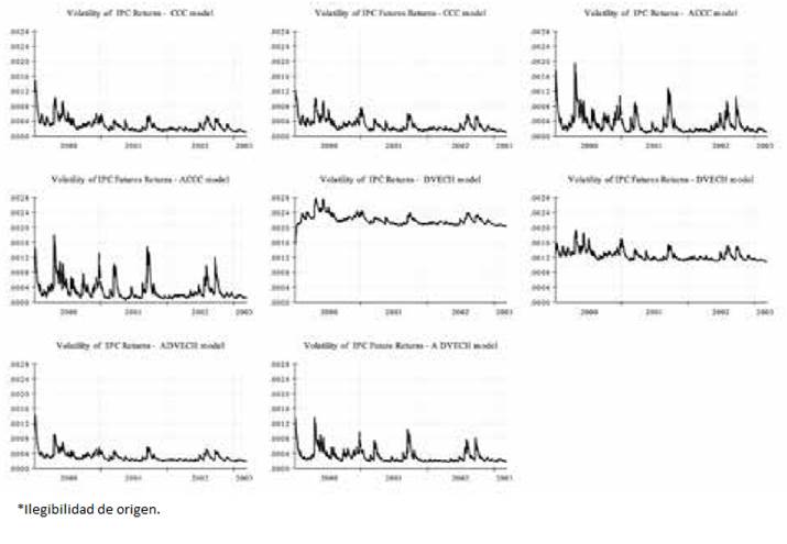
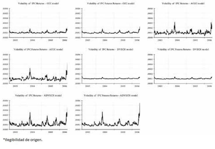
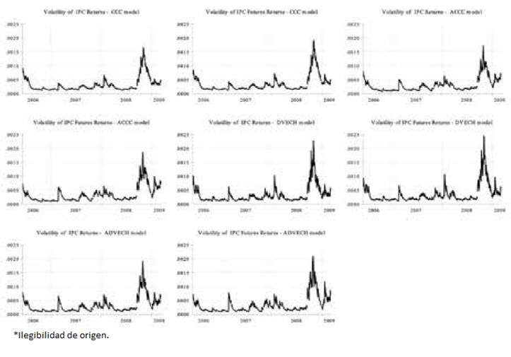
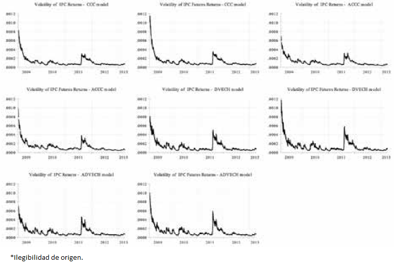
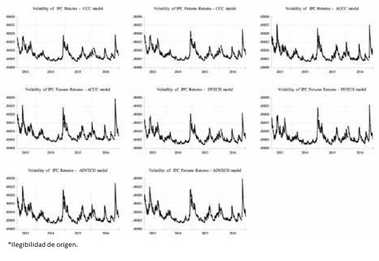
While the econometric analysis was performed for both the symmetric and asymmetric version of the DVECH and the CCC GARCH models, the following results (Tables 6-9) refer only to the Asymmetric DVECH and Asymmetric CCC models (the estimation output of the two symmetric models is available upon request from the authors), however, a graphical representation of the conditional variances of all four models is included as the Appendix. A visual representation of the effect of including the asymmetric response adjustment or not can be observed for both the DVECH and the CCC model in Figures A.1 through A.6. According to Figure A.1, conditional volatilities estimated for both the yields of the IPC and the yields of their futures contract are very similar for the full period, for the different models. They all capture the decline in volatility associated with the end of the dot.com bubble; the sharp rise in volatility associated with both the preamble and full manifestation of the Subprime Mortgages Crisis, as well as with the Sovereign Debt Crisis in the Eurozone. However, it is interesting to note that the maximum volatility is detected at different dates for each model, a situation that is observed in the same way for all the subperiods’ estimates. Also, the CCC and ACCC models show lower levels of conditional volatility and a smoother profile than their counterparts, the DVECH models. DVECH models estimated for the performance of the IPC and its futures contract during the first subperiod show very high conditional volatility levels compared to the other models, notably for the yields of the underlying. During subperiod 2, the opposite occurs, the estimated volatility of these models is the lowest, but, like the rest of the models, they capture the rising volatility at the end of that subperiod. The estimates for subperiods 3, 4 and 5 show similar behavior: all DVECH models produce higher conditional volatility estimates.
Table 6 Coefficients of the Asymmetric DVECH Model.
| Equation | Variable | FS | SP1 | SP2 | SP3 | SP4 | SP5 | |
|---|---|---|---|---|---|---|---|---|
| Mean Equations | Coint. Eq. (CE) | LIPC-1 | 1.000 | 1.000 | ||||
| LIPCF-1 - | 1.006*** | -1.006*** | ||||||
| C | 0.068 | 0.072 | ||||||
| LRIPC | CE | -0.033* | 0.324*** | |||||
| LRIPC-1 | 0.174*** | 1.132*** | 0.053 | -0.187 | 0.891*** | 0.415*** | ||
| LRIPC-2 | 0.260*** | -0.196*** | 0.115 | 0.050*** | 0.619*** | |||
| LRIPCF-1 | -0.098** | -0.021* | 0.031 | 0.210 | 0.126*** | 0.659*** | ||
| LRIPCF-2 | -0.256*** | 0.065*** | -0.151 | -0.076*** | -0.709*** | |||
| C | 0.000*** | 0.175*** | 0.001*** | 0.000 | 0.086*** | 0.164*** | ||
| LRIPCF | CE | 0.119*** | 0.508*** | |||||
| LRIPC-1 | 0.419*** | 0.410*** | 0.148 | -0.050 | 0.329*** | -0.169*** | ||
| LRIPC-2 | 0.366*** | -0.378*** | 0.206 | -0.187*** | 0.350*** | |||
| LRIPCF-1 | -0.331*** | 0.736*** | -0.031 | 0.073 | 0.687*** | 1.245*** | ||
| LRIPCF-2 | -0.352*** | 0.213*** | -0.219 | 0.163*** | -0.443*** | |||
| C | 0.000*** | 0.164*** | 0.001*** | 0.000 | 0.089*** | 0.184*** | ||
| Variance Equations | LRIPC | M | 0.000*** | 0.000*** | 0.000*** | 0.000*** | 0.000*** | 0.000*** |
| A1 | 0.037*** | 0.037*** | -0.011*** | 0.013 | 0.043*** | 0.044*** | ||
| D1 | 0.075*** | 0.055*** | 0.050*** | 0.125*** | 0.030*** | 0.055*** | ||
| B1 | 0.913*** | 0.866*** | 0.944*** | 0.885*** | 0.909*** | 0.898*** | ||
| LRIPCF | M | 0.000*** | 0.000*** | 0.000*** | 0.000*** | 0.000*** | 0.000*** | |
| A2 | 0.013*** | 0.007 | -0.011*** | 0.001 | 0.032*** | 0.036*** | ||
| D2 | 0.109*** | 0.181*** | 0.051*** | 0.150*** | 0.049*** | 0.053*** | ||
| B2 | 0.919 | 0.854 | 0.943 | 0.889 | 0.910 | 0.909 | ||
| Covariance | M | 0.000*** | 0.000*** | 0.000*** | 0.000*** | 0.000*** | 0.000*** | |
| A12 | 0.025*** | 0.022*** | -0.010*** | 0.008 | 0.038*** | 0.039*** | ||
| D12 | 0.092*** | 0.105*** | 0.049*** | 0.136*** | 0.038*** | 0.054*** | ||
| B12 | 0.916*** | 0.860*** | 0.941*** | 0.886*** | 0.908*** | 0.903*** | ||
| AdjR2_ols | 0.940359 | 0.902991 | 0.938196 | 0.957329 | 0.962232 | 0.967173 | ||
| AdjR2_As.dvech_1 | 0.003266 | 0.967051 | 0.010453 | 0.006116 | 0.995999 | 0.972142 | ||
| AdjR2_As.dvech_2 | 0.004720 | 0.967591 | 0.021515 | 0.007639 | 0.995600 | 0.969190 |
Note: *** = 1% significance; ** = 5% significance; * = 10% significance.
Source: Analysis formulated by the authors using data from Bloomberg.
Table 7 System Residual Portmanteau Tests for Autocorrelations, Corresponding to the Asymmetric DVECH Model Estimation.
| Adj Qstat Prob. | Full sample | Subperiod 1 | Subperiod 2 | Subperiod 3 | Subperiod 4 | Subperiod 5 |
|---|---|---|---|---|---|---|
| Lag 1 | 0.0001*** | 0.4695 | 0.7590 | 0.4249 | 0.2748 | 0.7632 |
| Lag 2 | 0.0000*** | 0.7194 | 0.9453 | 0.3815 | 0.2881 | 0.0165** |
| Lag 3 | 0.0000*** | 0.8512 | 0.9490 | 0.4274 | 0.1974 | 0.0249** |
| Lag 4 | 0.0000*** | 0.2883 | 0.9629 | 0.6644 | 0.0859 | 0.0286** |
| Lag 5 | 0.0000*** | 0.2852 | 0.6610 | 0.5584 | 0.1163 | 0.0444** |
| Lag 6 | 0.0000*** | 0.4174 | 0.7403 | 0.5646 | 0.2157 | 0.0368** |
| Lag 7 | 0.0000*** | 0.2328 | 0.7990 | 0.6698 | 0.3031 | 0.0306** |
| Lag 8 | 0.0000*** | 0.2533 | 0.8553 | 0.7435 | 0.4356 | 0.0373** |
| Lag 9 | 0.0000*** | 0.2715 | 0.9136 | 0.8691 | 0.3218 | 0.0321** |
| Lag 10 | 0.0000*** | 0.2984 | 0.8688 | 0.8791 | 0.3643 | 0.0528* |
| Lag 11 | 0.0000*** | 0.1929 | 0.9002 | 0.9219 | 0.3498 | 0.0609* |
| Lag 12 | 0.0000*** | 0.2137 | 0.9555 | 0.8865 | 0.3579 | 0.0749* |
Conditional Correlation Orthogonalization (Doornik-Hansen)
Note: *** = 1% significance; ** = 5% significance; * = 10% significance
Source: Analysis formulated by the authors using data from Bloomberg.
Table 8 Coefficients of the Asymmetric CCC GARCH.
| Equation | Variable | FS | SP1 | SP2 | SP3 | SP4 | SP5 |
|---|---|---|---|---|---|---|---|
| Coint. Eq. | LIPC-1 | 1.000 | 1.000 | ||||
| (CE) | LIPCF-1 | -1.006*** | -1.006*** | ||||
| C | 0.068 | 0.072 | |||||
| LRIPC | CE | 0.257*** | 0.336*** | ||||
| LRIPC-1 | -0.059 | 0.206** | 0.168 | -0.171 | -0.201 | -0.623*** | |
| LRIPC-2 | 0.074 | -0.079 | -0.079 | 0.024 | -0.060 | -0.151 | |
| LRIPCF-1 | 0.157*** | 0.177 | 0.240* | 0.667*** | |||
| LRIPCF-2 | -0.061 | -0.001* | 0.001*** | -0.070 | 0.084 | 0.142 | |
| C | 0.000 | 0.000 | 0.000 | 0.000 | |||
| LRIPCF | CE | 0.340*** | 0.391*** | 0.302** | 0.496*** | ||
| LRIPC-1 | 0.144*** | -0.241*** | -0.181 | -0.037 | 0.207 | -0.244 | |
| LRIPC-2 | 0.123** | 0.103 | 0.122 | 0.024 | |||
| LRIPCF-1 | -0.035 | -0.001** | 0.001*** | 0.038 | -0.163 | 0.287 | |
| LRIPCF-2 | -0.107** | -0.131 | -0.102 | -0.038 | |||
| C | 0.000 | 0.000*** | 0.000*** | 0.000 | 0.000 | 0.000 | |
| VarLRIPC | M | 0.000*** | 0.000*** | 0.000*** | 0.000*** | ||
| RESID-1 | 0.002 | -0.011 | -0.044*** | -0.020** | 0.008 | -0.008 | |
| TARCH-1 | 0.082*** | 0.223*** | 0.099*** | 0.120*** | 0.039*** | 0.095*** | |
| GARCH-1 | 0.952*** | 0.873*** | 0.896*** | 0.937*** | 0.952*** | 0.938*** | |
| VarLRIPCF | M | 0.000*** | 0.000*** | 0.000*** | 0.000*** | 0.000*** | 0.000*** |
| RESID-1 | 0.002 | -0.012 | -0.044*** | -0.019** | 0.001 | -0.001 | |
| TARCH-1 | 0.086*** | 0.254*** | 0.089*** | 0.128*** | 0.049*** | 0.085*** | |
| GARCH-1 | 0.950*** | 0.862*** | 0.931*** | 0.932*** | 0.951*** | 0.935*** | |
| Correl | R1,2 | 0.974*** | 0.955*** | 0.966*** | 0.979*** | 0.981*** | 0.986*** |
Note: *** = 1% significance; ** = 5% significance; * = 10% significance.
Source: Analysis formulated by the authors using data from Bloomberg.
Table 9 System Residual Portmanteau Tests for Autocorrelations, Corresponding to the Asymmetric CCC Model Estimation.
| Adj. Qstat Prob. | Full-sample | Subperiod 1 | Subperiod 2 | Subperiod 3 | Subperiod 4 | Subperiod 5 |
|---|---|---|---|---|---|---|
| Lag 1 | 0.0525* | 0.7386 | 0.9819 | 0.2492 | 0.9926 | 0.9612 |
| Lag 2 | 0.0021** | 0.6908 | 0.9871 | 0.5606 | 0.9938 | 0.9592 |
| Lag 3 | 0.0044** | 0.8553 | 0.9756 | 0.7232 | 0.6014 | 0.3644 |
| Lag 4 | 0.0001*** | 0.1807 | 0.9850 | 0.9097 | 0.4549 | 0.3029 |
| Lag 5 | 0.0000*** | 0.1057 | 0.7287 | 0.8706 | 0.6121 | 0.3128 |
| Lag 6 | 0.0000*** | 0.2439 | 0.8571 | 0.8414 | 0.6735 | 0.0960* |
| Lag 7 | 0.0000*** | 0.2520 | 0.9045 | 0.9160 | 0.7501 | 0.0912* |
| Lag 8 | 0.0000*** | 0.2471 | 0.9482 | 0.9469 | 0.8301 | 0.1616 |
| Lag 9 | 0.0000*** | 0.2526 | 0.9747 | 0.9817 | 0.7709 | 0.1070 |
| Lag 10 | 0.0000*** | 0.3317 | 0.9357 | 0.9854 | 0.8347 | 0.1749 |
| Lag 11 | 0.0000*** | 0.1436 | 0.9540 | 0.9891 | 0.7975 | 0.2471 |
| Lag 12 | 0.0000*** | 0.1647 | 0.9810 | 0.9704 | 0.8662 | 0.3364 |
Conditional Correlation Orthogonalization (Doornik-Hansen).
Note: *** = 1% significance; ** = 5% significance; * = 10% significance.
Source: Analysis formulated by the authors using data from Bloomberg.
The decision to omit the tables that report the output of the symmetric version of both models responds to space limitations and to the fact that the results obtained with models that take into account a differentiated response of volatility to positive and negative innovations are considered to have a better adjustment (e.g., Brooks et al., 2002; Brooks, 2003), which is clearly reflected in the figures included in the Appendix. Furthermore, the performance evaluation of the dynamic hedge ratios strategy is reported only for the Asymmetric CCC model, which offers the best adjustment of the two, as will be explained below based on the output of the estimations reported in Tables 7 and 9.
Table 6 shows the estimated Asymmetric-DVECH model’s coefficients for the full-period and the five subperiods determined by the analysis of structural breaks of the series. The coefficients of the cointegrating equation in the mean equation are significant for the full sample and for Subperiod 3, confirming the previous findings of cointegration between the variables, and fully consistent with previous studies that document the relationship between an underlying asset and its corresponding future contract. Also, the coefficients of the terms inside each cointegrating equation match the expectations mentioned earlier for equation [3], since β1 is close to -1 and β2 is close to 0 in both subperiods. Lastly, the GARCH, the Asymmetric term, and the Correlation parameter are significant in all the variance equations.
To test for the presence of autocorrelation in the residuals of the models presented in table 6 above, the results of the System Residual Portmanteau Test for Autocorrelation are presented in Table 7, below. For the full period, all the autoregressive terms are statistically significantly different from zero, i.e., there is strong evidence of autocorrelation problems. However, when the same test is carried out for the subperiods, the first four are free from autocorrelation, while the fifth is affected by significant autocorrelation in eleven of the twelve lags.
e Asymmetric CCC models’ coefficients for the five sub-periods are reported in Table 8. The coefficients of the cointegrating equation as a term in the mean equations, α1 and α2, are significant for the full sample and for subperiods 3, which confirms our previous findings of cointegration between the two variables when tested in those time periods. This is consistent with previous studies that document the relationship between the underlying asset and its corresponding future contract. Also, the coefficients of the terms inside each cointegrating equation match the expectations mentioned earlier for equation [3], since β1 is close to - 1 and β2 is close to 0 in both subperiods. Lastly, the GARCH, the Asymmetric term, and the Correlation parameter are significant in all the variance equations.
Table 9 shows the Portmanteau test for autocorrelation using Conditional Correlation orthogonalization. Similar to the case of the Asymmetric DVECH model, the Asymmetric CCC model autocorrelation tests show the coefficients are significant for the first twelve lagged residuals of the full sample. However, in all the subperiods, autocorrelations are not significantly different from zero at a 5 percent significance level. That fact makes the Asymmetric CCC model vastly superior to the Asymmetric DVECH model and justifies the decision to further develop the dynamic optimal hedge ratios using the Asymmetric CCC.
The conditional variance and covariance series from each sub-period’s estimated Asymmetric CCC model are next used to calculate the dynamic hedge ratio as in equation [1]. However, the constant hedge ratios for each subperiod using the OLS approach described earlier are also obtained and used as a benchmark. These Constant Hedge Ratios are reported in Table 10, below.
Table 10 Constant Hedge Ratios Estimated by OLS.
| Period | βols |
|---|---|
| Full-sample (12/30/1999-12/30/2016) | 0.9448 |
| Subperiod 1 (12/30/1999-3/12/2003) | 0.9419 |
| Subperiod 2 (3/13/2003-6/13/2006) | 0.9752 |
| Subperiod 3 (6/14/2006-3/09/2009) | 0.9391 |
| Subperiod 4 (3/10/2009-4/11/2013) | 0.9366 |
| Subperiod 5 (4/12/2013-12/30/2016) | 0.9508 |
Source: Estimation formulated by the authors using data from Bloomberg.
Next, we obtain the returns of theoretical portfolios that follow each of the three hedging strategies: the naive,2 constant and dynamic hedge ratios, in all three cases using equation [11]. This equation follows our previous assumption that the hedge ratio is calculated using the forecasted variance and covariance for the following time-period. In the cases of the portfolios following either the constant or the dynamic hedge ratio strategy, a time-series of their returns was constructed for the full sample by appending the results corresponding to each subperiod’s model, to compare them with the naive strategy and calculate their performance for the whole period of analysis.
Table 11 reports the performance of the four strategies, including the no-hedge scenario, used as a benchmark to measure the benefits from each of the hedging strategies for the full sample and for each subperiod. Additionally, Table 11 reports the results of an out-of-sample performance evaluation of the four strategies for the next 20 trading days after December 30th, 2016, the end of the sample period. The performance of each strategy during the forecast period is simulated as follows: a) using the previous sub-period (SP5) hedge ratio in the case of the OLS strategy; b) using the conditional hedge ratio obtained from the last observation of the SP5 for the first day of the forecast period, and the following daily changing hedge ratios based on the previous day conditional variance and covariance values obtained from the Asymmetric CCC model; or c) using the 1:1 ratio in the case of the naive hedge strategy.
Table 11 Portfolio Volatility and Range of Returns for Each Hedging Strategy.
| Strategy | Period | σrp | Min. Return | Max. Return |
|---|---|---|---|---|
| No Hedge (LRIPC) | Full sample | 1.3226% | -8.3% | 10.4% |
| SP1 | 1.6850% | -8.3% | 7.0% | |
| SP2 | 1.0421% | -4.4% | 3.2% | |
| SP3 | 1.8279% | -7.3% | 10.4% | |
| SP4 | 1.1099% | -6.1% | 6.2% | |
| SP5 | 0.8923% | -4.7% | 3.5% | |
| Forecast horizon | 0.9389% | -1.4% | 2.2% | |
| Naïve (1:1 hedge) | Full sample | 0.3315% | -4.8% | 2.5% |
| SP1 | 0.5337% | -4.8% | 2.5% | |
| SP2 | 0.2602% | -2.2% | 1.1% | |
| SP3 | 0.3948% | -2.5% | 2.2% | |
| SP4 | 0.2278% | -2.1% | 0.9% | |
| SP5 | 0.1678% | -1.1% | 0.8% | |
| Forecast horizon | 0.1313% | -0.2% | 0.3% | |
| OLS (constant for each subperiod) | Full sample | 0.3226% | -4.4% | 2.2% |
| SP1 | 0.5245% | -4.4% | 2.2% | |
| SP2 | 0.2589% | -2.2% | 1.2% | |
| SP3 | 0.3774% | -2.4% | 2.0% | |
| SP4 | 0.2156% | -1.6% | 0.8% | |
| SP5 | 0.1616% | -1.0% | 0.8% | |
| Forecast horizon | 0.1254% | -0.2% | 0.3% | |
| CCC (dynamic and asymmetric) | Full sample | 0.3213% | -4.1% | 2.8% |
| SP1 | 0.5205% | -4.1% | 2.8% | |
| SP2 | 0.2572% | -2.2% | 1.1% | |
| SP3 | 0.3786% | -2.3% | 2.0% | |
| SP4 | 0.2143% | -1.0% | 0.8% | |
| SP5 | 0.1631% | -1.0% | 0.8% | |
| Forecast horizon | 0.1300% | -0.2% | 0.3% |
Source: Estimation formulated by the authors using data from Bloomberg.
The volatility reduction achieved following each strategy, relative to the un-hedged case is reported in Table 12. The three hedge strategies prove very effective as they all significantly reduce volatility compared to the un-hedged scenario, but the Asymmetric CCC strategy is found to be more effective than the other two for the whole period. The naive strategy is always the least successful of the three strategies, and the Asymmetric CCC strategy shows better results than the OLS approach for three of the five sub-periods. In any case, the Asymmetric CCC strategy is also very close to the best performing strategy in the other two sub-periods, as well as during the forecast horizon. Any of the three optimal hedge ratio strategies seems to work much better for the forecast horizon than for any of the past five sub-periods; however, the length of the observation period is much shorter than in the case of any of the sub-periods and, of course, the whole period, so these results should be taken with some caution.
Table 12 Volatility Reduction of Each Hedging Strategy Vs. the Unhedged Case.
| Naïve | OLS | Asymmetric CCC | |
|---|---|---|---|
| F. sample (12/30/1999 12/30/2016) | 74.93% | 75.61% | 75.70% |
| Subperiod 1 (12/30/1999 3/12/2003) | 59.65% | 60.35% | 60.65% |
| Subperiod 2 (3/13/2003 6/13/2006) | 80.33% | 80.42% | 80.56% |
| Subperiod 3 (6/14/2006 3/09/2009) | 70.15% | 71.46% | 71.38% |
| Subperiod 4 (3/10/2009 4/11/2013) | 82.77% | 83.70% | 83.79% |
| Subperiod 5 (4/12/2013 12/30/2016) | 87.31% | 87.78% | 87.67% |
| Forecast horizon (20 days) | 90.07% | 90.52% | 90.17% |
Source: Estimation formulated by the authors using data from Bloomberg.
The predominance of the Asymmetric CCC dynamic hedging strategy is, finally, corroborated using the following portfolio risk performance measures: a) Value at Risk (VaR), defined as the loss level that should not be exceeded with a certain confidence level (α) during a certain period of time (t); b) Expected Shortfall (ES), meaning the average loss over a certain time-period (t), assuming that it is greater than the (1- α) percentile of the loss distribution. VaR and ES complement each other, and, in both cases, a small magnitude is preferred. Two more risk measures considered are the c) mean and d) maximum Absolute Deviations (AD mean and AD max, respectively) between the observations and the quantiles, as in McAleer and Da Veiga (2008). The last portfolio risk performance measure is e) the Average Quantile Loss (LAQ), which is a goodness-of-fit measure for VaR, with smaller values indicating a better fit, as in Gonzalez-Rivera et al. (2004).
As reported in Table 13, according to all five risk measures, the Asymmetric CCC-based hedge ratio strategy formulation proves superior to the OLS and the Naive models estimated for the full sample, and for all sub-periods, except the last one. In subperiod 5, OLS results are marginally better according to the ES and AD mean risk measures. The Naive model is consistently the worst model in most cases, with only two instances in which it is superior to the OLS model, but not to the Asymmetric CCC model in any subperiod. Overall, we consider the Asymmetric CCC to provide the best hedge. Notwithstanding, the OLS model is a close second and has the advantage that, as a passive approach, its transaction costs should give it a practical advantage over the former.
Table 13 In-sample Risk Measures.
| Period | Model | VaR | ES | AD mean | AD max | LAQ |
|---|---|---|---|---|---|---|
| Full-sample | As. CCC | 0.0074 | 0.0085 | 0.0070 | 0.0338 | 0.0002 |
| OLS | 0.0075 | 0.0086 | 0.0075 | 0.0367 | 0.0002 | |
| Naïve | 0.0077 | 0.0085 | 0.0083 | 0.0400 | 0.0002 | |
| SP1 | As. CCC | 0.0120 | 0.0137 | 0.0140 | 0.0292 | 0.0004 |
| OLS | 0.0122 | 0.0139 | 0.0155 | 0.0321 | 0.0004 | |
| Naïve | 0.0124 | 0.0142 | 0.0166 | 0.0354 | 0.0004 | |
| SP2 | As. CCC | 0.0059 | 0.0068 | 0.0063 | 0.0157 | 0.0002 |
| OLS | 0.0060 | 0.0069 | 0.0063 | 0.0157 | 0.0002 | |
| Naïve | 0.0060 | 0.0069 | 0.0066 | 0.0163 | 0.0002 | |
| SP3 | As. CCC | 0.0088 | 0.0101 | 0.0046 | 0.0144 | 0.0002 |
| OLS | 0.0088 | 0.0101 | 0.0050 | 0.0149 | 0.0002 | |
| Naïve | 0.0092 | 0.0105 | 0.0048 | 0.0155 | 0.0002 | |
| SP4 | As. CCC | 0.0049 | 0.0056 | 0.0025 | 0.0055 | 0.0001 |
| OLS | 0.0050 | 0.0057 | 0.0027 | 0.0109 | 0.0001 | |
| Naïve | 0.0053 | 0.0061 | 0.0028 | 0.0156 | 0.0001 | |
| SP5 | As. CCC | 0.0038 | 0.0044 | 0.0015 | 0.0063 | 0.0001 |
| OLS | 0.0038 | 0.0043 | 0.0014 | 0.0067 | 0.0001 | |
| Naïve | 0.0039 | 0.0045 | 0.0015 | 0.0072 | 0.0001 |
Source: Estimation formulated by the authors using data from Bloomberg.
As a general conclusion, it may be said that the hedge ratios built with the Asymmetric CCC model effectively reduce volatility and the complementary risk measures beyond the improvements obtained with a constant hedge ratio, either naive or OLS-based estimations, as could be expected in the implementation of hedging strategies from more sophisticated techniques. Our findings reinforce the confidence that practitioners may have in the use of futures contracts for hedging diversified portfolios of Mexican stocks, and provide authorities in charge of the MexDer with an empirical example of the usefulness of such contracts when hedging strategies are supported with adequate econometric estimations of the optimal hedge ratio at all times. As the country’s financial markets become more diversified and sophisticated, there will be a growing need for many other types of futures contracts, as well as for a careful analysis of different dynamic hedging strategies. That reality creates attractive areas of research that have great practical usefulness and provide theoretical challenges for the profession.
Conclusion
This paper compares the hedging performance of four different strategies in the combination of the IPC and its corresponding futures contract, the IPCF: a) a No-hedge strategy; b) a Naive hedge ratio (1 to 1); c) a Constant Hedge ratio, obtained with an OLS model; and d) a dynamic hedge ratio, obtained using a CCC Asymmetric Bivariate GARCH model. The estimation of the dynamic hedge ratio needed to implement strategy d) required the selection of a conditional variance/covariance model, so the initial analysis included a BEKK model, as well as asymmetric CCC and DVECH models. The choice of the asymmetric bivariate CCC-GARCH model to estimate dynamic hedge ratios for a portfolio that contains the IPC and its futures contract was based on the overwhelming evidence found in the literature on the better performance of asymmetric conditional variance models over their non-asymmetric counterparts (Brooks et al., 2002). However, the choice of the Asymmetric CCC model over the Asymmetric DVECH model was also based on the comparison of both models’ output, and the confirmation that the presence of significant autocorrelation in the residuals of the estimated models was less of a problem in the case of the former model.
The three hedging strategies prove to be very effective and to reduce volatility significantly when compared with the un-hedged alternative, but the Dynamic Asymmetric CCC strategy is confirmed to be more effective than the Naive or constant hedge ratio strategies for the whole period. The Naive strategy consistently proves to be the least successful of the three strategies, and the Asymmetric CCC strategy shows better results than the fixed hedge ratio (OLS) approach for three of the five sub-periods. Nevertheless, the Asymmetric CCC strategy is also very close to the best performing strategy in the other two sub-periods, as well as during the forecast horizon. The three statistically based strategies work much better for the forecast horizon than for the full sample period or any of the five sub-periods; however, the length of the forecast period is much shorter than in the case of any of the sub-periods and, of course, of the whole period, so these results should be taken with some caution. By contrasting different strategies that a typical investor can follow regarding the utilization of the IPCF to hedge a diversified portfolio of Mexican stocks, the conclusion of this work’s results is that any hedging strategy, including the naive strategy that assumes investors hedge on a one-to-one basis (one futures contract per unit of exposure), results in much less volatility in the returns of a Mexican stock portfolio than the no-hedge strategy.
From the comparison of two possible MGARCH modeling approaches, the DVECH and the CCC models, we confirm that both present serious autocorrelation problems for the full-sample period. However, once the sample is segmented according to previously identified structural breakpoint dates, while the DVECH model still presents autocorrelation in the estimation residuals, the CCC model (conventional and asymmetric) overcomes the autocorrelation problem. Finally, when comparing the two CCC versions of the model, the Asymmetric CCC is a better choice because its performance is superior in terms of volatility reduction, in-line with previous literature. To corroborate the high quality of the Dynamic Asymmetric CCC-built hedge strategy, we compare the different portfolios’ performance using several risk measures (VaR, ES and LAQ), and confirm that it is superior in most subperiods. However, the OLS approach is a close second and, as a passive approach, it may have a definitive advantage when considering transaction costs inherent to a dynamic hedging strategy.
The necessary conditions for an emerging capital market to thrive include the existence of increasingly sophisticated and liquid markets for financial securities and commodities. The institutional conditions for those markets to thrive are difficult to build but cannot be considered a matter of choice as they are an important building block that helps firms implement risk management strategies and control their exposure against unfavorable market conditions. The need for more complete derivatives markets that provide economic agents with a sufficient variety of contracts to implement investment risk management strategies and design portfolios that better respond to their risk-return preferences and objectives should clearly be a priority of emerging markets. At present, few emerging markets have modern and well-functioning derivatives markets. The MexDer represents a step in the right direction towards the modernization and sophistication of the Mexican financial market. Important environmental changes, including financial deregulation and the reform of the Mexican pension system, created individual retirement accounts managed by institutional investors (Afores) instead of the traditional “pay-as-you-go” system. This represents an exceptional opportunity for derivative contracts and the consolidation of the MexDer. There is a growing interest from other interested parties (agricultural product producers, mining companies, etc.) to have access to mechanisms that will help them to compensate uncertainty in the price of their product. Stimulating the development of a derivatives market is consistent with the objective of economic modernization and better conditions for producers across the economy. In addition, as part of that process, a better knowledge of the characteristics and functioning of the MexDer futures contracts represents a valuable insight that deserves further attention and study.