


 nova página do texto(beta)
 Inglês (pdf)
 Artigo em XML
 Referências do artigo
 Enviar este artigo por email
 Citado por SciELO
  Similares em
SciELO
Similares em
SciELO 
 Permalink
Introduction
As indicated by Baffes, Kose, Ohnsorge and Stocker (2015), in recent decades, the oil sector has reflected instability in international oil prices, which have been more representative since 2004 and respond to various factors, such as the policies of the Organization of Petroleum Exporting Countries (OPEC), geopolitical tensions, imbalances between supply and demand in international markets and others. Likewise, Sadorsky (1999) states that extreme fluctuations in oil prices have an impact on economic activity and significantly affect movements in the stock market.
Therefore, facing an uncertain and volatile scenario, how can we find accurate models that facilitate better risk management? VaR, as a standard for measuring and evaluating risk, and CVaR, as a coherent measure of risk, are used to estimate losses (maximum probable and expected) given a level of confidence on a time horizon and under normal market conditions that present adverse price movements. However, it has been shown that normality is not the best adjustment for financial instruments, resulting in better approximations of alternative distributions, as in the case of the GH family, proposed by Barndorff-Nielsen in 1977. This class of distributions is defined by five parameters; by fixing the parameter λ = -1⁄2, the NIG distribution is obtained. He exposed the capability of NIG distribution to model heavier tails than that of normal distribution, a fact commonly found in return data series (Barndorff-Nielsen, 1977, 1997).
Within that environment, we will focus this study on VaR and CVaR estimates in BRIC country oil companies, comparing the precision of both values and considering NIG as an alternative to normal distribution. According to Núñez, Contreras-Valdez, Ramírez-García and Sánchez-Ruenes (2018), adjustment of data series of the main indexes of BRIC economies to NIG distribution during periods of volatility has proven to be a better option than normal distribution.
It should be noted that the choice of distribution for calculating VaR and CVaR impacts the estimate of the quartiles that determine the risk. Moreover, better adjustment of the empirical data to a specific distribution type enables construction of functions that more accurately estimate the risk given the conditions of uncertainty and volatility.
Some recent studies have applied distributions from the GH family to adjust the returns in prices of commodities such as oil and gold. This is the case of Mota and Mata (2016), who have adjusted the prices of various petroleum mixtures to a GH distribution in two periods: 2010-2013 and 2014-2015. The results showed that empirical data better fit this class of distributions.
Regarding gold returns, data (from 1991-2017) have been adjusted to some GH distributions to estimate the VaR, obtaining better approximations than with normal distribution (Shen, Meng and Meng, 2017; Shen, Meng, Guo, Zhao, Ding and Meng, 2017).
The hypothesis for this paper is that in times of instability, when using NIG distribution, risk estimation through VaR and CVaR quantification on equity price returns of BRIC oil companies is greater, compared to normal distribution.
This research differs from existing literature on the parametric estimate of VaR through alternative NIG distribution of the equity returns of oil companies in BRIC economies, as most papers found in the oil sector focus on estimating the risk measures of crude blend prices assuming traditional distributions as the norm.
The paper is organized in five sections: Section 2 presents and discusses the concepts and methods for estimating VaR and CVaR, as well as a description of NIG distribution. In section 3 we present the methodology applied to the data to estimate VaR and CVaR through alternative distributions: normal and NIG; the results are presented in section 4, and finally, section 5 discusses the conclusions.
I. Literature Review
The Basel Committee on Banking Supervision (1996) requires that financial institutions, such as banks and investment firms, comply with the capital requirement based on VaR estimation. An incorrect VaR estimate results in sub-optimal resource allocation.
Yamai and Yoshiba (2005) studied and compared VaR and CVaR risk measures. We approach the concepts presented below from that compilation.
Following Artzner, Delbaen, Eber and Heath (1997), VaR is defined as the maximum probable loss of a portfolio or financial instrument in a given time horizon for a level of confidence under normal market circumstances because of adverse movements in prices.
Definition 1. Given a time interval [t; T], the relative change in the value of a portfolio in a given time horizon τ = T - t is defined as:
where Π(t) = 1n V(t), V(t) represents the value of the portfolio at time t. If
X = ΔΠt (τ), then X: Ω→
i.e.:
from which the following is derived:
from the VaR definition, it is possible to obtain the VaR given the cumulative distribution function of the portfolio returns:
where Fx(x) = P (X ≤ x) is the cumulative distribution function of the portfolio returns over a period and f x (x) is the probability density function of X. Then:
That is, the VaR is the quantile q of Fx. Therefore, the essence of the VaR calculation is the estimation of the lower quantiles of the cumulative distribution function of the portfolio returns, which in practice is unknown (Artzner, Delbaen, Eber and Heath, 1999).
VaR estimation methods suggest different ways of constructing this function. The most common are the parametric method, the historical simulation and the Monte Carlo simulation.
Lauridsen (2000) presented an overview of the main VaR estimation methods, comparing their performance, advantages and drawbacks.
VaR Estimation by Historical Simulation
In this method, historical financial data produce future behavior information. Therefore, it is possible to use financial data history to obtain significant predictions of future performance.
Historical simulation is a relatively simple method that is easy to implement and has the advantage of not needing to assume that returns follow a normal distribution.
In general, the historical method depends on observed data, so if the sample size is not large enough, there is a greater chance that the VaR estimate lacks precision.
Various articles, such as Hendricks (1996) and Barone-Adesi et al. (2000), provide a detailed discussion of the historical simulation approach.
VaR Estimation by Monte Carlo Simulation
Through this method, recently addressed by Hong, Hu and Liu (2014), an approximation of the expected return performance of a portfolio or financial instrument is obtained by means of simulations that generate random trajectories of the returns of the portfolio or financial instrument, considering certain initial assumptions about volatilities and correlations of risk factors.
Parametric VaR
The parametric method is used under the assumption that the observed data follow some rules or models with unknown parameters. We use these data to obtain parameter estimates and apply the rule or model established to calculate the VaR, as Mentel (2013) pointed out. The parametric method offers two approaches: unconditional and conditional.
Unconditional Approach
In this method, the assumption is that the financial returns in each period of time are independent and identically distributed random variables (IID) that follow a multivariate normal distribution. However, various investigations show that multivariate Gaussian distribution cannot explain some properties of the empirical distribution of financial data. For example, Fama (1965), Hull and White (1998) point out that changes in several market variables (stock prices, prices of zero coupon bonds, exchange rates, commodity prices, etc.) are leptokurtic, that is, there are too many values close to the average and too many in the extreme tails. These changes increase the probability of very large and very small movements in the value of market variables and decrease the probability of moderate movements. Therefore, there is not enough evidence to support the Gaussian hypothesis, so we propose a distribution with different characteristics.
Conditional Approach
It admits that time series of financial returns depend on past information. Traditionally, the Autoregressive Moving Average Model (ARMA) describes a series dependence, where we obtain a stationary series. However, ARMA models assume that the variance is constant, and given that generally speaking the volatility of financial time series is not constant, these models are not suitable to use with them.
The most popular of several studies aimed at finding models that describe the volatility variable in time, a common characteristic of financial returns, is Engle’s Autoregressive Conditional Heteroscedasticity model (ARCH, 1982), where the variance conditioned on past information is not constant and depends on the square of past innovations. Subsequently, Bollerslev (1986) generalized arch models by proposing the Generalized Conditional Autoregressive Heteroscedasticity (GARCH) models. Here, the conditional variance depends not only on the squares of perturbations, as in arch models, but also on the conditional variances of previous periods. Both models may be combined with the ARMA model, obtaining the ARMA-ARCH and ARMA-GARCH models.
In the standard GARCH model, widely used today, we assume that observed data fits a Gaussian distribution. For many financial return series, however, the Gaussian distribution is inadequate, since it does not consider leptokurtosis.
Strengths and Weaknesses of VaR
VaR is a popular risk measure, because it can quantify the market risk of a financial institution by calculating a unique numerical value. This value is the maximum possible loss of a portfolio or financial instrument in a given period of time, for a certain level of confidence (Barone-Adesi, Giannopoulos and Vosper, 2000). At the same time, one of its disadvantages is that, by definition, it ignores losses whose probability of occurrence is less than that chosen as the level of confidence in the estimation. For these reasons, Bali affirms that standard VaR provides an inadequate estimation of losses during periods of high volatility such as those corresponding to financial crises (Bali, 2007).
On the other hand, Artzner, Delbaen, Eber and Heath (1999) indicate that one of its main disadvantages is that it is not a coherent measure of risk and non-convex. A measure of risk is coherent if it satisfies the axioms of monotonicity, subadditivity, positive homogeneity and invariance under translations.
Conditional Value at Risk
An alternative coherent risk measure is CVaR, introduced by Artzner, Delbaen, Eber and Heath, defined here as the expected loss that exceeds the VaR. In general, CVaR provides the conditional expectations of loss above the VaR. Some other names for CVaR are Expected Shortfall, Mean Excess Loss, Beyond VaR, Tail VaR, Conditional Loss and Expected Tail Loss.
CVaR provides better adjustment and consistency in the estimation of risk with respect to the VaR, since it complements p-value information provided by the VaR, becoming very useful with asymmetric distributions (Artzner, Delbaen, Eber and Heath, 1997).
Rockafellar and Uryasev (2002) show that the CVaR is a coherent measure of risk, as well as the significant advantages of this methodology with respect to the traditional VaR. On the other hand, Kibzun and Kuznetsov (2003) mention that under normal conditions, CVaR is a convex function with respect to the positions taken, which allows the construction of an efficient optimization algorithm. Peña (2002) indicates that despite the advantages of VaR over CVaR, both are complementary measures; that is, if the objective of VaR is to control market risk under normal conditions, the objective of CVaR is to control market risks in extreme conditions. In addition, it is possible to establish a relationship between VaR and CVaR if a specific parametric distribution is assumed. For the specific case of normality, the VaR and CVaR are similar.
Therefore, we can consider the use of CVaR as a complement to VaR. So, if the objective of the VaR is to control market risk under normal conditions, the objective of the CVaR is to control market risks in extreme conditions.
Currently, both risk measures are widely used both in the field of research and in empirical studies and applications.
Portfolio Optimization
Regardless of whether we apply VaR or CVaR to measure the risk of a portfolio or financial instrument, one of the natural objectives of risk management is portfolio optimization. In Markowitz Portfolio Theory, the concepts of correlation and covariance are key elements of the model. In addition, it introduced the concept of diversification, that is, the addition of certain assets to an investment portfolio, to decrease risk.
The objective of Markowitz (1952) was to find the optimal allocation for each investment instrument, minimizing variance (considered as the risk measure) subject to a condition on the expected return; that is, the investor wants to obtain the highest return and is adverse to risk. For Markowitz, a portfolio is considered efficient if it provides the maximum possible return for a given level of risk, or equivalently, if it provides the lowest possible risk for a specific level of profitability.
Thus, we can say that an optimal portfolio is a combination of financial instruments that represent a risk-return ratio that maximizes investor satisfaction. Here we assume that individual assets follow Gaussian distributions and there is a correlation matrix for the dependence between the assets.
Variance may be replaced by other risk measures such as VaR and CVaR. Since VaR is not a consistent measure, though, it is difficult to find the optimal portfolio for minimizing it. Gaivoronski and Pflug (2005) propose an approach to VaR using a soft measure called SVaR (local minimizer) that filters irregularities locally. The approach, however, is too complex.
On the other hand, CVaR is a coherent and convex measure, so a unique global minimizer may be found. Rockafellar and Uryasev (2002) point out a simple way to optimize a portfolio by minimizing CVaR, which enables transforming the problem into a classic linear programming problem. Recently, various studies that extend this model have come to light, including Andersson et al. (2001); Charpentier and Oulidi (2008); Glasserman et al. (2002); and Krokhmal et al. (2001).
All these authors, however, use the historical approach to calculate portfolio allocation. Therefore, if there is not enough historical data, risk may be severely underestimated. Another drawback is that they do not address the dependence of the historical data series.
As already mentioned, the financial data series is not perfectly independent, since there is a correlation between the returns on different actions and different types of risks. Therefore, it is essential to describe such risk management correlations and establish the necessity of knowing about joint distribution of financial data.
Previously, among the assumptions about the joint distribution function was multivariate normal distribution. With this distribution, dependency is described by the correlation matrix, and obtaining the risk measure is simple (Markowitz, 1952). However, this assumption does not work well for financial data.
In addition to normal distribution, another approach will be used in this paper to describe financial series: NIG distribution, which is a particular case of the family of GH distributions that will be described in detail in the next section.
II. Methodology
For the purpose of this study, we used daily data from Bloomberg on equity from the following BRIC crude oil producing companies:
Petróleo Brasileiro S. A. in Brazil; pjsc Rosneft Oil Company, in Russia; Oil & Natural Gas Corporation Limited, Oil India Limited, Gail India Limited and Cairn India Limited, in India; and Kunlun Energy Company Limited, China Petroleum & Chemical Corporation and China National Offshore Oil Corporation, in China.
The 2004-2017 period selected for the series of data included several destabilizing events that occurred, such as:
• The price bubble caused by the growth in oil demand from China and India and fixing of oil level by producing countries (2004 - 2007)
The financial crisis (2007 - 2008)
The rise in prices due to the reactivation of economies and increase in demand by emerging economies (2009 - 2013)
The drop in oil prices as of 2014 due to oversupply and weakening demand in the oil markets, as well as Saudi Arabia’s decision to maintain its oil production levels.
Due to data availability, with some companies we only considered certain events, as is the case of Rosneft, where we obtained data from 2006 and Oil India, with information as of 2009 (Baffes, Kose, Ohnsorge and Stocker, 2015).
With each equity series, we calculated the logarithmic return for daily data as an approximation to a continuous series. The equation to obtain logarithmic returns is:
where:
ri represents the return of the index on the day.
Pi represents the closing level of the index at day i.
Pi-1 is the closing level of the index at day i - 1.
Descriptive Statistics
Skewness and kurtosis were calculated for each equity series in order to validate distributions with higher skewness values, either positive or negative. So we can expect that the empirical data do not correspond to a normal distribution.
The following table presents some statistics for the series considered:
Table 1 Descriptive Statistics
| Country | Company | Equity | Mean | Variance | Skewness | Kurtosis |
|---|---|---|---|---|---|---|
| Brazil | Petrobras | PETR3 BZ | 0.0001 | 0.0010 | -0.017 | 3.925 |
| PETR4 BZ | 0.0001 | 0.0010 | -0.2081 | 4.7732 | ||
| Russia | Rosneft | ROSN RX | -0.0001 | 0.0008 | 1.3606 | 36.2001 |
| India | ONGC | ONGC IN | 0.0001 | 0.0005 | 0.1444 | 4.8558 |
| ONGC IB | 0.0001 | 0.0005 | -0.1443 | 4.9206 | ||
| ONGC IS | 0.0001 | 0.0005 | -0.1517 | 4.8777 | ||
| Oil India | OINL IN | 0.00004 | 0.0003 | -0.0039 | 2.2466 | |
| OINL IB | 0.00004 | 0.0003 | 0.0895 | 2.5768 | ||
| OINL IS | 0.00004 | 0.0003 | -0.0039 | 2.2466 | ||
| GAIL | GAIL IN | 0.0003 | 0.0006 | -0.1290 | 13.3321 | |
| GAIL IB | 0.0003 | 0.0006 | -0.1205 | 14.0466 | ||
| GAIL IS | 0.0003 | 0.0006 | -0.1813 | 13.2171 | ||
| CAIRN | CAIRN IN | 0.0002 | 0.0007 | -0.3793 | 4.7279 | |
| CAIRN IS | 0.0002 | 0.0007 | -0.3793 | 4.7279 | ||
| China | CNPC | 135 HK | 0.0005 | 0.0006 | -0.0446 | 5.8627 |
| SINOPEC | 386 HK | 0.0002 | 0.0006 | 0.1606 | 5.2435 | |
| CNOOC | 883 HK | 0.0004 | 0.0006 | 0.1702 | 5.1632 |
* High Kurtosis values appeared in every data series distribution. Source: own elaboration in R Software with data from Bloomberg.
By analyzing the excess of kurtosis, different behavior from the normal distribution is noted, so the presence of heavy tails is expected.
Normality Test
When we use the Anderson-Darling and Shapiro-Francia normality tests, the null hypothesis of normality may be rejected. In this case, the proposed NIG distribution becomes a candidate to fit the empirical data. We establish both normality tests as follows:
H0: We confirm a sample resulting from a normal distribution.
Ha: We discard a sample that comes from a normal distribution, H0 is discarded.
For the null hypothesis test, the p-value of each data series was set using both Anderson-Darling (1954) and Shapiro-Francia (1972) proofs, with a significance level of 0.05, so, if p - value ≥ 0.05 the null hypothesis is not rejected.
Shapiro-Francia Test
The normality test developed by Shapiro and Francia (1972) is an approximate and simplified version of the Shapiro Wilk test to prove the normality of a larger series of data. The test parameter is obtained by calculating the slope of the regression line by simple least squares, i.e.,
Anderson Darling Test
The Anderson-Darling (1954) criteria test the hypothesis that a data series comes from a population that adheres to a continuous Cumulative Distribution Function (CDF). We can express the test as follows:
Normal Inverse Gaussian Distribution
As mentioned before, multiple studies prove that NIG distribution fits the financial series. Barndorff-Nielsen (1997) defined this kind of distribution:
where
and
where K1 is the modified Bessel
function of third order and index 1. Also, α, β, μ and
δ are parameters, satisfying 0 ≤ |β| ≤
α, μ ∈
Parameters α and β determine the shape, and μ and δ scale the distribution. Parameter α denotes the flatness of the density function, i.e. a high value of α means a greater concentration of the probability around μ. Parameter β defines a kind of skewness of the distribution. When β = 0, the NIG distribution is symmetric around the mean. A negative value represents a heavier left tail. Parameter δ describes the distribution scale, and parameter μ is responsible for the distribution density shift.
Goodness of Fit Tests
By simulating a vector with the obtained parameters, we test the similarity of both distributions with Kolmogorov-Smirnov and Anderson-Darling criteria in which the p-values correspond with the acceptance region of the null hypothesis. So according to the statistical tests, it can be stated that NIG distribution is capable of modeling returns even during a period of economic crisis.
VaR and CVaR Estimates
From definition 1 we can obtain the VaR knowing the cumulative distribution function of the asset’s returns:
where
Assuming that the distribution of asset returns is normal, described by mean parameters μ and standard deviation σ, the VaR calculation consists of finding the qth percentile of the standard normal distribution zq:
where X* = zqσ + μ, and Φ(z) is the standard normal density function, N(z) is the cumulative normal distribution function, X is the asset performance, g(x) is the normal distribution function of the yields with mean μ and standard deviation σ, and X* is the minimum yield at confidence level 1 - q.
The CVaR of X at level 1-q is defined as the expected loss, given that this loss exceeds the VaR, that is:
The CVaR complements the information provided by the VaR. As mentioned earlier, it is very useful when we have asymmetric distributions, as well as being an excellent risk management tool, applicable in distributions with peaks.
III. Results
Through the results obtained by calculating the descriptive statistics of the series, we observed that all series have high kurtosis values, except in Oil India Limited, with a value less than 3. In both tests, we assumed a significance level of 0.05 and obtained a p-value less than 2.2 × 10⁻¹⁶ in all cases, meaning the null hypothesis of normality is rejected.
In addition, we applied the Anderson-Darling and Shapiro-Francia normality tests to confirm that the series were not normal. Then we fitted the series with a member of the GH family: NIG distribution.
Having proven the no-normality of equities return distribution and the excess kurtosis obtained from the descriptive statistics of the series, NIG distribution can model the empirical data to obtain a distribution that better describes the empirical data series.
Maximum Likelihood Estimation (MLE) was applied for the NIG parameters. Although other methods could have been used, the selected algorithm solves the maximization problem through numerical methods. The table below shows the parameters obtained using R software.
Table 2 NIG Parameters
| Country | Company | Equity | α | β | δ | μ | N |
|---|---|---|---|---|---|---|---|
| Brazil | Petrobras | PETR3 BZ | 27.7696 | -2.5228 | 0.0259 | 0.0025 | 3463 |
| PETR4 BZ | 27.8003 | -1.2370 | 0.0265 | 0.0013 | 3463 | ||
| Russia | Rosneft | ROSN RX | 27.4717 | 1.1942 | 0.0185 | -0.0009 | 2870 |
| India | ONGC | ONGC IN | 45.2371 | -0.2926 | 0.0237 | 0.0003 | 3480 |
| ONGC IB | 44.6404 | -0.0489 | 0.0228 | 0.0002 | 3480 | ||
| ONGC IS | 45.3151 | -0.2969 | 0.0238 | 0.0003 | 3480 | ||
| Oil India | OINL IN | 62.0062 | -0.9141 | 0.0200 | 0.0003 | 2049 | |
| OINL IB | 58.4773 | 0.5684 | 0.0183 | -0.0001 | 2049 | ||
| OINL IS | 62.0062 | -0.9140 | 0.0200 | 0.0003 | 2049 | ||
| GAIL | GAIL IN | 39.9015 | 0.7049 | 0.0228 | -0.0001 | 3480 | |
| GAIL IB | 39.6728 | 0.9236 | 0.0221 | -0.0002 | 3480 | ||
| GAIL IS | 40.0952 | 0.8189 | 0.0228 | -0.0002 | 3480 | ||
| CAIRN | CAIRN IN | 34.5280 | -1.5625 | 0.0238 | 0.0012 | 2549 | |
| CAIRN IS | 34.5280 | -1.5625 | 0.0238 | 0.0012 | 2549 | ||
| China | CNPC | 135 HK | 29.6789 | 1.8679 | 0.0191 | -0.0007 | 3454 |
| SINOPEC | 386 HK | 35.2436 | 0.0443 | 0.0194 | 0.0002 | 3454 | |
| CNOOC | 883 HK | 35.2196 | 0.0726 | 0.0210 | 0.0003 | 3454 |
NIG parameters obtained for each series. Source: own elaboration in R Software with data from Bloomberg
With the estimated NIG parameters, we simulated a series with a particular NIG distribution in order to do a statistical analysis using a log-likelihood test to compare the similarity of the empirical data series with the simulated data series. Kolmogorov-Smirnov and Anderson-Darling tests were used for this purpose.
The results confirm the null hypothesis, i.e. the statistical similarity of empirical data and NIG distributions in all cases. Therefore, according to statistical criteria, NIG distribution can fit the equities return distribution.
Table 3 Likelihood Test (p-value)
| Country | Company | Equity | Kolmogorov-Smirnov | Anderson-Darling |
|---|---|---|---|---|
| Brazil | Petrobras | PETR3 BZ | 0.4789 | 0.4103 |
| PETR4 BZ | 0.5555 | 0.5466 | ||
| Russia | Rosneft | ROSN RX | 0.281 | 0.533 |
| India | ONGC | ONGC IN | 0.2888 | 0.3001 |
| ONGC IB | 0.8652 | 0.7755 | ||
| ONGC IS | 0.07921 | 0.08834 | ||
| Oil India | OINL IN | 0.3053 | 0.3152 | |
| OINL IB | 0.5496 | 0.5372 | ||
| OINL IS | 0.964 | 0.9378 | ||
| GAIL | GAIL IN | 0.1756 | 0.307 | |
| GAIL IB | 0.07921 | 0.06038 | ||
| GAIL IS | 0.7584 | 0.7136 | ||
| CAIRN | CAIRN IN | 0.4588 | 0.5876 | |
| CAIRN IS | 0.6752 | 0.6754 | ||
| China | CNPC | 135 HK | 0.2346 | 0.4428 |
| SINOPEC | 386 HK | 0.3269 | 0.414 | |
| CNOOC | 883 HK | 0.8926 | 0.8357 |
Both tests assume a significance level of 0.05, meaning that if p-value is greater than or equal to 0.05, the null hypothesis is not rejected; otherwise the alternative hypothesis is confirmed. Source: own elaboration with R Software using data from Bloomberg
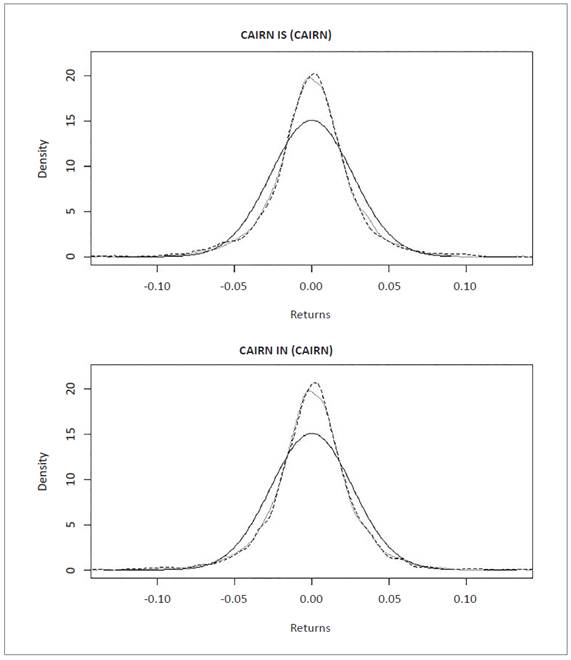
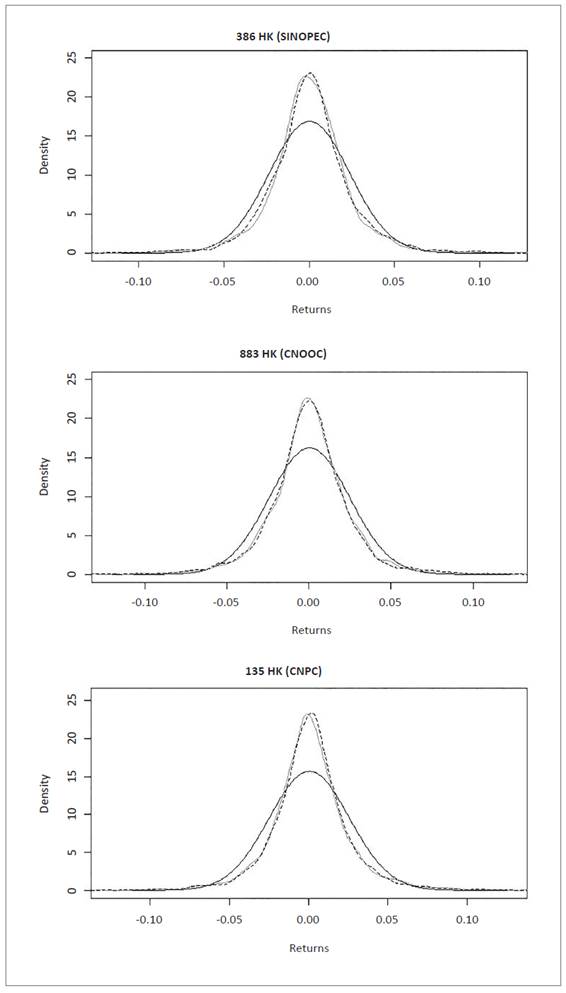
Quantitative results of the likelihood test between NIG simulation distribution and empirical data distribution can be observed graphically in the qualitative comparison of normal distribution (red), empirical data distribution (blue), and simulated NIG distribution (green), in the figures below.
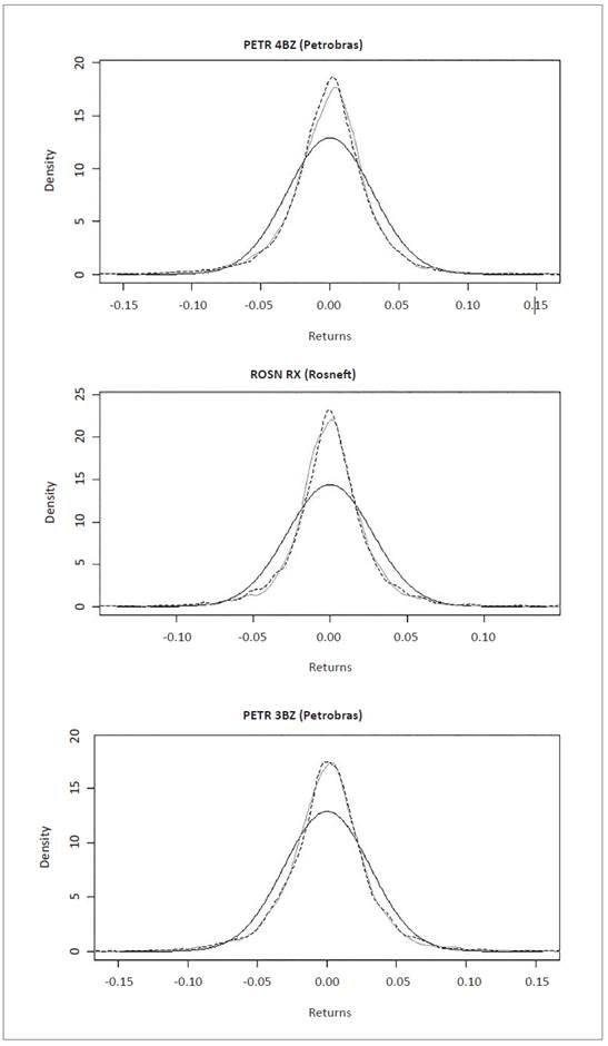
Distribution graphs show normal distribution (dark gray line), empirical data distribution (light gray line) and NIG simulat ed distribution (dashed line), for interpretation purposes. The graphs were generated with R software.
Figure 1 Normal, empirical and NIG data series distribution for equities in Petrobras and Rosneft companies. Source: own elaboration with R Software using data from Bloomberg.
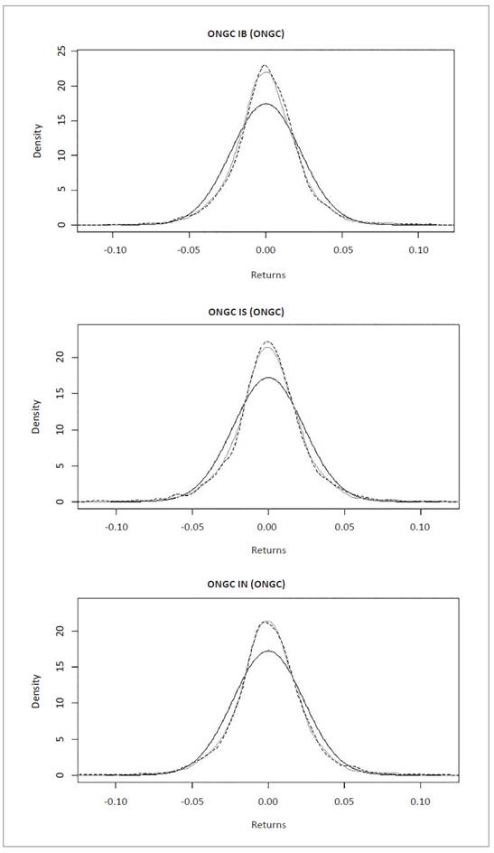
Distribution graphs show normal distribution (dark gray line), empirical data distribution (light gray line) and NIG simulated distribution (dashed line), for interpretation purposes. The graphs were generated with R software.
Figure 2 Normal, empirical and NIG data series distribution for equities in Oil & Natural Gas Corporation Limited (ONGC). Source: own elaboration with R Software using data from Bloomberg.
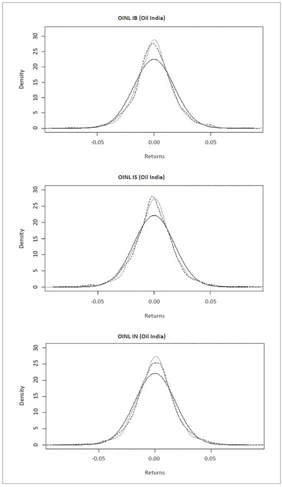
Distribution graphs show normal distribution (dark gray line), empirical data distribution (light gray line) and NIG simulated distribution (dashed line), for interpretation purposes. The graphs were generated with R software.
Figure 3 Normal, empirical and NIG data series distribution for equities in Oil India Limited (OINL). Source: own elaboration with R Software using data from Bloomberg.
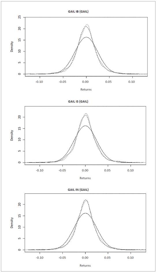
Distribution graphs show normal distribution (dark gray line), empirical data distribution (light gray line) and NIG simulated distribution (dashed line), for interpretation purposes. The graphs were generated with R software.
Figure 4 Normal, empirical and NIG data series distribution for equities in Gail India Limited. Source: own elaboration with R Software using data from Bloomberg.
Distribution graphs show normal distribution (dark gray line), empirical data distribution (light gray line) and NIG simulated distribution (dashed line), for interpretation purposes. The graphs were generated with R software.
Figure 5 Normal, empirical and NIG data series distribution for equities in Cairn India Limited. Source: own elaboration with R Software using data from Bloomberg.
Distribution graphs show normal distribution (dark gray line), empirical data distribution (light gray line) and NIG simulated distribution (dashed line), for interpretation purposes. The graphs were generated with R software.
Figure 6 Normal, empirical and NIG data series distribution for equities in Kunlun Energy Company Limited (CNPC), China Petroleum & Chemical Corporation (SINOPEC) and China National Offshore Oil Corporation (CNOOC). Source: own elaboration with R Software using data from Bloomberg.
We calculated Values at Risk and Conditional Values at Risk using R software, first considering a normal distribution and establishing the μ (mean) and σ (standard deviation) parameters indicated in Table 1. Then we used NIG distributions with the parameters α (distribution flatness), β (distribution skewness), δ (scale of the distribution) and μ (shift of the distribution) specified in Table 2.
Table 4 shows the values obtained, where in all cases we observe that VaR were less than CVaR when both were calculated with normal distribution. It also happened when we obtained the VaR and CVaR using NIG distribution. The VaR with normal distribution were less than CVaR with NIG distribution, and also CVaR with normal distribution were less than CVaR with NIG distribution, i.e.:
VaRnormal distribution < CVaRnormal distribution
VaRnig distribution < CVaR nig distribution
VaRnormal distribution < VaRnig distribution
CVaRnormal distribution < CVaRnig distribution
We thus confirmed that CVaR estimates provide higher values than VaR, which means an underestimation of the risk by VaR, compared to CVaR using both normal and NIG distributions.
In addition, in VaR and CVaR estimates, we observed that NIG distribution provides higher values than the estimates based on normal distribution, that is, the NIG distribution model provided estimates of the largest potential losses. Table 4. Values at Risk (VaR) and Conditional Values at Risk (CVaR).
Table 4 Values at Risk (VaR) and Conditional Values at Risk (CVaR).
| Country | Company | Equity | Normal distribution | NIG distribution | ||
|---|---|---|---|---|---|---|
| VaR | CVaR | VaR | CVaR | |||
| Brazil | Petrobras | PETR3 BZ | -0.0718 | -0.0822 | -0.0896 | -0.1178 |
| PETR4 BZ | -0.0720 | -0.0825 | -0.0877 | -0.1146 | ||
| Russia | Rosneft | ROSN RX | -0.0645 | -0.0739 | -0.0724 | -0.0962 |
| India | ONGC | ONGC IN | -0.0537 | -0.0615 | -0.0616 | -0.0784 |
| ONGC IB | -0.0530 | -0.0608 | -0.0609 | -0.0777 | ||
| ONGC IS | -0.0537 | -0.0616 | -0.0616 | -0.0784 | ||
| Oil India | OINL IN | -0.0418 | -0.0479 | -0.0481 | -0.0607 | |
| OINL IB | -0.0412 | -0.0472 | -0.0473 | -0.0601 | ||
| OINL IS | -0.0418 | -0.0479 | -0.0481 | -0.0607 | ||
| GAIL | GAIL IN | -0.0571 | -0.0655 | -0.0641 | -0.0823 | |
| GAIL IB | -0.0566 | -0.0649 | -0.0633 | -0.0815 | ||
| GAIL IS | -0.0571 | -0.0654 | -0.0639 | -0.0820 | ||
| CAIRN | CAIRN IN | -0.0614 | -0.0703 | -0.0738 | -0.0958 | |
| CAIRN IS | -0.0614 | -0.0703 | -0.0738 | -0.0958 | ||
| China | CNPC | 135 HK | -0.0586 | -0.0672 | -0.0687 | -0.0907 |
| SINOPEC | 386 HK | -0.0548 | -0.0628 | -0.0652 | -0.0853 | |
| CNOOC | 883 HK | -0.0568 | -0.0651 | -0.0672 | -0.0875 | |
Both VaR and CVaR measures obtained are higher, respectively, when NIG distribution is considered than the values calculated when normality is assumed. Source: own elaboration with R Software using data from Bloomberg.
Conclusions
This study provided evidence that in the equities of BRIC economy oil companies, the CVaR model used with NIG distribution provides the biggest estimate of potential losses, compared to the CVaR estimate considering normal distribution or a VaR with NIG or normal distribution. The results were obtained by quantifying the VaR and CVaR of the assets of oil producing companies in Brazil, Russia, India and China in volatile periods between 2004 and 2017. For the VaR and CVaR estimate based on NIG distribution, we obtained the parameters describing the function and confirmed that it adjusted the empirical data of the equity returns reasonably.
This represents a benefit by quantifying, with less underestimation, the risks that respond to the extreme price fluctuations associated with the oil sector, under a given level of confidence.
It is worth mentioning that it would be feasible to expand this research in the future and analyze VaR and CVaR performance using other heavier tail distributions, to explain stronger volatility movements. The study could also be extended to companies in other oil-producing countries, in order to analyze their equity variation in times of uncertainty and compare their statistical dependence with those studied in this paper.

