


Servicios Personalizados
Revista
Articulo
 Inglés (pdf)
 Artículo en XML
 Referencias del artículo
 Enviar artículo por email
Indicadores
-
 Citado por SciELO
 -
 Accesos
Links relacionados
-
 Similares en
SciELO
Similares en
SciELO
Compartir

 Permalink
Economía: teoría y práctica
versión On-line ISSN 2448-7481versión impresa ISSN 0188-3380
Econ: teor. práct no.37 México jul./dic. 2012
Upper and Lower Bounds for Capital and Wages*
Alberto Benítez Sánchez ** Alejandro Benítez Sánchez ***
** Departamento de Economía, UAM–Iztapalapa. E–mail: abaxayacatl3@gmail.com. View my research on my SSRN Author page: http://ssrn,com/author=1717472.
*** Departamento de Ingeniería Industrial, Instituto Tecnológico de Tijuana. E–mail: thesphinx423@hotmail.com
*Fecha de recepción: 11/07/2011.
Fecha de aprobación final: 17/05/2012.
RESUMEN
El artículo estudia la división de un sistema de producción en los departamentos I y II e introduce una división posterior del departamento I en un sector homotético y otro complementario. Muestra la existencia de cotas superiores e inferiores no triviales para el acervo de capital y para el salario que dependen de esta división, con lo cual contribuye, entre otros resultados, a explicar la casi linealidad de la curva salarios–ganancia encontrada en algunos estudios empíricos.
Palabras clave: teoría del capital, distribución del ingreso, Marx, Sraffa, curva salarios–ganancia.
Clasificación JEL: B2, B5, P1.
ABSTRACT
The paper considers the division of a production system into departments I and II introducing a further division of department I into a homothetic and a complementary sector. It shows the existence of nontrivial upper and lower bounds for the capital stock and the wages that depend on this division contributing, among other results, to explain the quasilinearity of the wage–profit curve found in some empirical researches.
Keywords: capital theory, income distribution, Marx, Sraffa, wage–profit curve.
JEL classification: B2, B5, P1.
The division of a production system according to the final use given to the products of each enterprise, either as means of production or consumption goods, was originally introduced by Smith (1981: 288) and reformulated by Marx (1992: 471) who, like his predecessor, employed this division mainly to study the reproduction of the economic system. On the other hand, von Neuman (1945) built a homothetic production system to study economic growth in a general equilibrium model and, from a perspective inspired in Ricardo (2004), Sraffa (1960) built another system of this type to study the relations between prices and income distribution. The important analytical tools introduced by these authors have been incorporated in numerous publications but, to our knowledge, they have been employed separately despite the proximity of the themes treated in many of the researches.1
In this paper, we define the aggregates of production processes just mentioned within a model of single–product industries with no fixed capital in such a way that they result complementary. With this purpose, we first divide this system into departments i and ii introducing a further division of department i into a homothetic sector and the rest of this department, to which we refer to as the complementary sector. A division of production into three parts is thus established with a corresponding division of labor into three quantities, represented synthetically by means of a vector l =(lh, lc,l II), whose coordinates are the quantities of labor occupied in the homothetic sector, the complementary sector and department ii, respectively. The vector, under certain election criterion specified in third section, is unique for each production system and constitutes a useful tool to study the capital stock and the wage measured with the net product, respectively KS and w, as functions of the profit rate (r).2 This conclusion is based on the results that are presented along the paper in the order indicated.
In the first section, we expose a model originally published in Benítez (2009) whose most peculiar trait is to include all possible distributions of wage's payment between the start and the end of production.3 In second section, we establish the division into departments and prove that, given l and the maximum rate of profit (R), KS depends only on the proportion capital/(total product) in department I (cI). In third section, we accomplish the further division of department I and prove that, given l and R, cI depends only on the proportion capital/(total product) in the complementary sector (cc), a result that, together with the one just indicated implies that the same is valid for KS.
Moreover, in fourth section it is shown that, for each R, the possible values of KS are contained in the space limited by the curve 1/r, the vertical straight line of abscise R and the two axes, in relation to which two important results are presented. According to the first one for each r ∈ [0, R] and for each number pertaining to the interval [0, 1/r] there is at least one production system for which KS(r) is equal to that number. Consequently, as shown in sixth section, for each number pertaining to the interval [0, 1] there is at least one production system where profits (KS (r) r) are equal to that number for any r ∈ [0, R]. Therefore, the graphics of the functions KS (r) and those of the wage–profit curves not only belong respectively to the space just indicated and to the rectangle of diagonal S (R) = [(0, 1), (R, 0)], something already known, but also cover these surfaces entirely, a conclusion not previously published to our knowledge. This situation gives relevance to the second result: each vector l determines a nontrivial lower bound for the capital stock valid for the set C (R), integrated by all the production systems sharing the same R. On its turn, this bound implies an upper bound for the wage (w) that is presented in sixth section.
Given the last result, one may expect that l also determined an upper bound for KS valid for C(R), but in fifth section, we prove that this is not the case. For this reason, in the same section we consider a family of subsets Cm(R) ⊃ C(R) defined in such a manner that, for each m > 0, Cm(R) contains all the elements of C(R) except a part of those where the following takes place: for some r* ∈ [0, R], when r changes from r* to R, the capital stock of the complementary sector diminishes in an amount greater than or equal to m times the simultaneous increase in its profits. The definition is helpful in the study of those production systems where, for empirical or theoretical reasons, the possibility of such a reduction in the capital stock may be excluded. In this regard, the case m = 1 is particularly interesting, as argued in sixth section Also in this section, we prove that for each m, l determines an upper bound for the capital stock valid for Cm (R) which, together with the lower bound already mentioned, permits one to establish an estimation of KS(r) whose precision may be great for certain values of r.
On the basis of the last result, in seventh section, a lower bound for the wage is determined for each set Cm (R) which, together with the upper bound already mentioned, permits one to estimate w(r) with an accuracy that may be high for certain levels of m, l and r. Finally, despite the fact that no empirical applications are included in this paper, in the final remarks section it is argued that the results presented here may have empirical relevance. We shall add that the roman character appearing in some statements indicates the section of the "Appendix where the reader may find the corresponding proof.
1. THE MODEL
The model represents a productive system integrated by n industrial branches, each producing a particular type of good labeled by an index i or j, so that i, j = 1, 2, …, n. I will refer to a set { j1, j2,…, jd,…, jD} as a D set if it contains D different goods. To simplify, I will also refer to the indexes as goods. All the production processes are simultaneous and of equal duration, the quantities of each good are measured with the amount produced of the corresponding good, and the quantities of salaries with the amount of salaries paid.4 For each pair (i, j) of indexes, aij and lj represent respectively the quantities of i and of salaries consumed in the j industry during the period considered to produce one unit of j; for each j they verify lj >0, aij ≥ 0 ∀ i and aij > 0 at least for one i. If the assumption is made that each quantity of salaries pays an equal quantity of labor, lj may also be interpreted as the quantity of labor consumed in the j th industry; however, this is not required for the purposes of this paper. For each j, the price of good j in units of salary is pj and r is the rate of profit of the period. A fraction t of the wages is paid at the beginning of production in every industry and the rest at the end, the cost of labor in each branch j is then equal to lj t (1 + r) + lj(l– t) =lj(1+ tr). In these conditions, if the rate of profit is the same in every branch, the prices and costs of production are related by the following equation system:

We will say that (1) is viable if in every D set the sum of the quantities of each good belonging to D that are consumed directly in the production of the goods of D is not greater than 1 and is less than 1 for at least one of the goods. Consequently, every D set verifies that Σdaijd≤ 1 for each i ∈ D and Σdaijd < 1 for at least one i∈ D. I assume that every economy considered in this work is viable, which, together with the other assumptions already made permit us to verify the following propositions for every t.
Theorem 1.I There is an interval [0, R] such that: a) R is independent of t and 0 < R < + ∞, b) for each r ∈ [0, R], the solution of (1) is unique and strictly positive, c) pj (r) is a monotonous increasing function for every j, d) at least one price tends to infinity when r tends to R, e) for each r ∈ [0, R], the quotient pi (r)lpj(r) is independent of t ∀ (i, j).
For each i, ci = 1 – Σjaij represents the quantity of good i produced as surplus over the amount of the same good consumed as a means of production, as (1) is viable ci ≥ 0 ∀ i and ci > 0 for at least one i. Summing up the n equations of (1), we obtain ΣjΣiaijpi (1 +r) + Σj lj (1 + tr) = Σjpj. Substituting Σj lj and Σjpj with their respective equivalents 1 and ΣjΣiaijpi + Σjcjpj in the previous equation yields ΣjΣiaijpi(1 + r) + (1 + tr) = ΣjΣiaijpi+ Σjcjpj and consequently:

The first term on the left–hand side of this equation is the amount of profits obtained with the means of production and the second one that of wages together with the profits corresponding to the wages advanced. As the value of the collection of goods on the right–hand side is equal to the net income of the society, we will refer to this collection as the real income.5 Let

The first function represents the capital stock (equal to the cost of the means of production), the second one the wage and the third one the capital (equal to the amount invested), each variable being measured with the real income. Using this notation we can write (2) in the following forms:

Dividing every term on the right–hand side of (3.a) by a price pb arbitrarily chosen yields KS=ΣjΣiaij(pi/pb)/Σjcj(pj/pb). This expression and e) from Theorem 1 imply that KS is independent of t. To simplify, I will assume in the next four sections that t = 0 and its other possible values will be considered only in seventh section. Under this assumption, the real income is equal to net product and for this reason, we will talk only about the last one in the corresponding sections.
II. DEPARTMENTS I AND II
Each industry i produces a certain quantity ci of consumption goods and another quantity 1 – ci of means of production. Therefore, we can represent its activity by means of two equations, one for each part of it, establishing the following equation systems:

The first system represents the production of capital goods and the second one that of consumption goods, named by Marx (1992:47) respectively dpartments I and II of production. If no industry belongs to the two departments either ci = 0 or ci = 1 for each i, naturally in this cases ci = 0 for at least one i and n > 1. Adding up the equations in each system yields, respectively, the following equations ΣjΣi(1 – ci)aijpi(1 + r) +Σj (1 –ci) lJ= Σj (1 – ci)pj and ΣjΣiclalJpl (1 + r) + ΣjcilJ= Σjctpi. To simplify, I will introduce the variables pI = Σj (1 – ci)pj, cI = ΣjΣi(1 – ci) alJpi/pI , lI = Σj(1 – ci)lJ, PII = Σjcipj and lII= 1 – lI. The quotient cI indicates the fraction of the production of department I consumed in the same department, as the rest of its production is consumed in department II and the total labor is employed in the two departments, we can write the preceding equations sum under the following forms:


Using this notation, the capital stock may be represented by means of the quotient pI/pII. Substituting the denominator in this fraction on the left–hand side of (6) gives pI /[(1– cI)pI (1 + r) + 1 –lI] =1/[(1 – cI)(1+ r) + (1 – lI)/pI]. On the other hand, solving (5) yields pI = lI/[1 – cI(1 + r)] and substituting pI according to this result on the right–hand side of the preceding equation, we get 1/{(1– cI)(1 +r) + (1–lI)[1– cI (1 + r)]/lI}=lI/{lI(1–cI)(1 + r) + (1 – lI)[1–cI(1 + r)]}= lI /{lI + lIr – cIlI (1 + r) + 1 –cI(1 + r) – lI + lIcI(1 + r)]}. Simplifying the last expression, we obtain:

This formula shows that, given r and lI, the capital stock depends only on cI. For this reason, in the next section we will study in more detail how this variable is determined.
III. THE HOMOTHETIC AND COMPLEMENTARY SECTORS
Let A = [aij], A* = [aji] and λA represent the Frobenius root of A. From the assumptions adopted, it follows that 0 < λA < 1, as shown in Benítez (2009). Therefore, according to Theorem 7 in Chapter 13 of Gantmatcher (1966), there is at least one vector q ≥ 0, q ≠ 0 such that A*q = λAq. As the magnitude of q may be fixed arbitrarily, we will assume, for reasons indicated below, that a q has been chosen satisfying the following conditions: a) the magnitude of q is such that min{1 –ci–qi= 0 |i = 1, 2,…, N} and b) q is one of the vectors maximizing the sum Σjqjlj. After q has been determined, multiplying each equation j of (1) by the corresponding factor qIresults in the following system:

This system is homothetic, a condition characterized by the fact that the proportion between the quantity of each good used as a means of production and the quantity produced of the same good is the same for all the goods, implying that KS is constant. Indeed, in (8) this proportion is equal to ΣjΣiqjaij pi/Σjqjpj permuting the indexes i and j in the numerator, we can express the function as ΣiΣjqiajipj/Σjqjpj= ΣjΣiqiajipj/Σjqjpj. Because A*q = λAq, for each j, we have Σiqiaji= λAqj and substituting in the preceding quotient, we get ΣiΣjqiajipj/Σjqjpj= ΣjλAqjpj Therefore:

On the other hand, the condition a) assumed to define q implies that system (8) is embedded in department I and, together with b) assures that, with regard to the quantity of labor employed, (8) is the greater homothetic system in this situation. As shown by Benítez (1986), there may be other homothetic systems, but for the purposes of this paper it is enough with the one satisfying conditions a) and b), to which I will refer as the homothetic sector.
According to the preceding definitions, for each j the part of the production of the jth industry included in department I may be divided into two fractions: the one integrating the homothetic sector, equal to qi, and the rest equal to 1 – ci – qi. A corresponding representation of department I by means of two equation systems can be formulated, (8) and the following system, to which I will refer as the complementary sector:
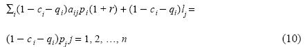
Therefore, this system is the complement of the homothetic system in department I. Despite the fact of being a residual determined by the two other systems just mentioned above, the complementary sector is relevant to our study, as will be shown. Summing up the equations of systems (8) and (10) result, respectively, in ΣjΣiqiaijpi(1 + r) +Σjqilj=Σjqipj and ΣjΣi (1 –ci,–qi)aijpi(1 + r)+Σj(1 –ci,–qi)lj=Σj(1 –c,–qi)pj. To simplify, I will introduce the variables ph = Σjqipj, lh=Σjqjlj,pc=Σj (1 –ci,–qi)pjand cc = ΣjΣi(1 –ci,–qi)aijpi/pc. As the quantity of labor employed in (10) is lI – lh, using this notation and (9), department I may be represented by means of the following system:

Solving each of these equations for the corresponding price yields ph = lh / [1 – λA(1 + r)] and pc = (lI – lh)/[1 – cc (1 + r)]. On the other hand, it follows from system (11) that cI = (λAph + cc pc) / (ph + pc ). Substituting prices in this equation for their equivalence, we get cI = {lhλA/[1 –λA(1 + r)] + (lI – lh )cc /[1 – cc (1 + r)]}/{lh/[1 –λA (1 + r)] + (lI – lh)/[1 – cc(1 + r)]} and multiplying both the numerator and the denominator in this formula by [1 – λA(1 + r)][1 – cc(1 + r)] yields:

This formula permits one to observe that cI∈ [ λA, cc] whenever λA≠ cc and also that given r, λA, lh and lI, cI depends only on cc, a variable that will be studied with more detail in the next sections. On the other hand, the preceding divisions permit one to define the vector l = (lh, lc, lII), which is unique for each system of type (1). The values of l are contained in the set S( l) = {l ∈ R3 | (lh, lc, lII) ≥ 0 and lh + lc + lII = 1} and may vary widely. Notwithstanding, if (1) is homothetic, then lI = R /(1 + R ), lII = 1/ (1 + R ) and, as in this case department I is also homothetic, the distribution of labor is given by:

IV. A LOWER BOUND FOR THE CAPITAL STOCK
To study the capital stock, the following proposition will be useful.
Lemma 1.II Let KSc be the proportion capitalI(net product) in the complementary sector, KS(R) and KSc(R), respectively, the limits of KS(r) and KSc(r) when r tends to R from below. Then:

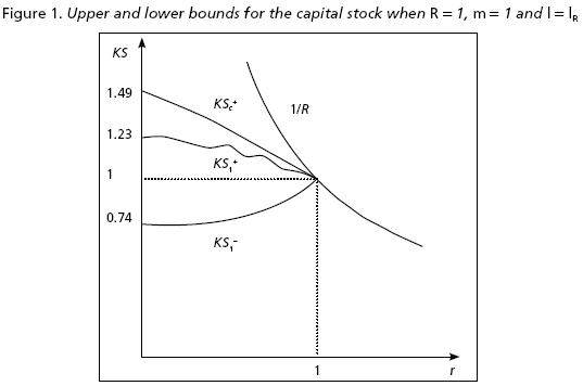
The graph of KS(R) as a function of R is the hyperbole equilateral shown in Figure 1.
Let GKS(R) = {(r, KS) | 0 ≤ r < R and 0 < KS < 1/r}∪{(R,1/R)}, according to (14.a) and (14.b) this set contains the graphs of KS(r) of all the systems (1) that share the same R. A natural question investigating the upper and lower bounds for KS is to ask if, given R, there are some other limits for KS apart from the hyperbole just mentioned and the horizontal axis, a question answered negatively in the following proposition.
Theorem 2.III Given R, ∀(r, T ) ∈ GKS(R), there is at least one system of type (1) for which KS(r) = T.
Accordingly, the ordinate of each point of GKS(R) is equal to the capital stock of at least one system of type (1) for the corresponding r. Therefore, given any R the magnitude of capital may be as close to zero as desired ∀ r ∈ [0, R]. Nevertheless, as it will be shown in this section, the distribution of labor among the departments and sectors of production determines a nonzero lower bound for the systems of type (1) sharing a given R. To show this, the following proposition will be useful, valid if lI – lh > 0.
Lemma 2.IV cI is a monotonous increasing function of cc.
It follows from this result that, given R and l, the smallest capital corresponds to the system of type (1) where cc is the smallest. Because in each industry at least one produced good is employed, this quantity is always greater than zero, but I will make it equal to zero in (12) to calculate the limit (cI–) of the proportion cI when cc tends to zero. After simplifying, one gets cI– = λA /{1 + (lI /lh – 1) [1 – λA (1 + r)]}. On the other hand, the first equation of (11) may be written in the form λA (1 + r) + lh /ph = 1. The second term, on the left–hand side tends to zero when r tends to R (see A.II in "Appendix") so that we have λA (1 + R) = 1 and:

Substituting in the previous expression gives cI– = 1/(1 + R) /{1 + (lI /lh – 1) [1 – (1 + r) /(1 + R)]} and multiplying everything by (1 + R), we obtain after simplifying:

According to (7), KS is a monotonous increasing function of cI. For this reason, to obtain a lower bound for the capital stock (KS –), it is enough to substitute this value of cI in (7) resulting in:

We may add that ∀ ∈ [0, R], this formula determines the greater lower bound for KS given R and l. This is because for every T > KS – it is possible to choose cc small enough for the resulting system to verify KS < T. Figure 1 presents an example of a lower bound for KS.
V. A FAMILY OF SUBSETS
For each R, let C(R) be the set of all the systems of type (1) that share the same R value. An important property of this set is presented next.
Proposition 1.V Given R and l, ∀ (r, T) ∈ GKS(R), there is at least one system of type (1) for which KS(r) > T.
This proposition implies that, given R, the vector l does not impose any upper limit on the capital stock. For this reason, in this section we are going to define a family of subsets of C(R), whose complement in C(R) may be reduced as much as desired and such that in each one of them a given vector l determines a nontrivial upper bound for the capital stock, as will be shown in the next section.
According to (15) (12) and (7), given l and R the capital stock depends only on cc, so that we will pay particular attention to this sector. It is convenient to observe that, if the capital stock is constant, KSc(r) ≤ 1/R ∀ r ∈ [0, R] according to (14.d). Then, if KSc(r*) > 1/R for a certain r* ∈ [0, R], necessarily KSc diminishes when r changes from r* to R. From equation (A.1) (see "Appendix"), it follows that when r = r*, the wage in the complementary sector, measured with the net product of the sector, is equal to [1 – KSc(r*)r*]. Let m be the reduction of the capital stock taking place when r changes from r* to R measured with the wage in r*, then m = [KSc(r*) – 1/R]/[1 – KSc(r*) r*]. Therefore, if for every r ∈ [0, R], the capital stock diminishes in an amount equivalent to m times the wage in r when the rate of profit changes from r to R, we have KSc(r) = m[1 – KSc(r)r] + 1/R and so:

For each couple (m, R) where R > 0 and m ≥ 0, let Cm(R) be the set of all the systems of type (1) for which KSc (r) is less than the value determined by (18) ∀ r ∈ [0, R]. We may ask if for every m ≥ 0 the amount of capital determined by (18) corresponds to at least one system of type (1) and also if for every system of type (1) there is an m ≥ 0 such that the capital stock is less than the value determined by (18) for every r ∈ [0, R]. Both questions receive an affirmative answer based on the following proposition.
Lemma 3.VI The family of functions (18) possesses the following properties: a) ∀ T ∈ [1/R,1/r [ and ∀ r ∈ [0, R] there is an m such that KS(r) = T, b) for every m > 0 the graph of (18) is below the hyperbole 1/R and c) for every r ∈ [0, R], KS(r) is a monotonous increasing function of m.
It is convenient to observe that according to (14.d) for every r* ∈ [0, R], when r changes from r* to R, the wage is reduced to a quantity equal to or greater than zero implying that the simultaneous increase in profits is smaller than or equal to the wage in r*. Consequently, in the systems verifying (18), the capital stock in the complementary sector diminishes with this change an amount equivalent to at least m times the increase in proits. For this reason, Cm(R) may be described as the set integrated by all the elements of C(R) except a part of those that, for some r* ∈ [0, R], when r changes from r* to R, the capital stock in the complementary sector diminishes in an amount equal to at least m times the simultaneous increase in profits. It follows from Lemma 3 that when m increases starting from zero the set Cm(R) ∩ C(R) grows continually from C0 (R), a set that includes only those systems where capital always grows when r changes from an r* ∈ [0, R] to R, and tend to be equal to Cm(R) when m tends to infinity. Finally, it is worth noting that a system of type (1) pertaining to a set Cm(R) satisfies a restriction regarding the relative price of the particular sets of goods integrated by the capital stock and the net product of the complementary sector but there is no other restriction on relative prices.
VI. AN UPPER BOUND FOR THE CAPITAL STOCK
For each m and for each r < R, (18) permits one to establish an upper bound cc+(r) for cc(r) valid for all the production systems pertaining to Cm(R). Indeed, KSc(r) = cc (r)/[1 – cc(r)]; it follows from this equation and (18) that an upper bound for cc (r) verifies cc+(r)/[1 – cc+(r)] = (1/R + m)/(1 + mr) implying that cc+(1 + mr) = (1 – cc+) (1/R + m), hence cc+[(1 + mr) + (1/R + m)] = (m + 1/R) and:

On its turn, this result permits one to establish the following upper bound for the capital stock:

obtained by substituting first cc for cc+ in (12) and the result (ci(cc+)) substitutes ci in (7).
To employ this formula, which calculates an upper bound for the capital stock of a particular system of type (1), an assumption is made about the smallest set Cm(R) containing the system, something that may depend on empirical or theore– tical considerations. In this regard, the set C1(R) has a special interest for the following reasons: a) it includes all the production systems where KSc(r) is a constant or a monotonous increasing function, b) it includes a part of those systems where KSc(r) is monotonously decreasing or not a monotonous function and c) it excludes only a part of those systems where for some r* ∈ [0, R], when r changes from r* to R, KSc(r) diminishes an amount at least equal to the corresponding increase in profits. It is to remark that in such cases the sum of capital plus profits, measured with the net product, either keeps constant or decreases. Formulas (17) and (20) permit one to estimate the capital stock as the average of the values determined by both, to which it corresponds a maximum error equal to one half of the difference between them. After simplifying, the following formula is established:

The value determined by (12) for (cI(cc+)) is always equal to 1/R when r = R. For this reason, the error in (21) is equal to zero in this case, a result indicating that it may be as small as desired for values of r sufficiently near to R. On the other hand, normally the error will be greater when r approaches zero. Figure 1 presents the graphs corresponding to (19) and (20) when m = 1, R = 1 and l = (1/4, 1/4, 1/2) is determined by (13).
VII. UPPER AND LOWER BOUNDS FOR WAGES
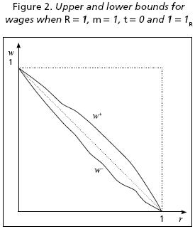
Let Gw(R) = {(r, w) | 0 < r < R and 0 < w < 1}∪{(0, 1), (R, 0)} this set contains all the possible graphs of w(r) and is equal to the interior points of a rectangle as those shown in Figures 2 and 3 plus the extreme points of S(R). We may ask if every point of this set pertains to the wage–profit curve of at least one system of type (1), an affirmative answer is given by the next proposition.
Theorem 3.VII Given R, ∀ r ∈ [0, R] and for every F such that 0 < F < 1, there is at least one system of type (1) for which w(r) = F.
Then, given R and r such that 0 < r < R, w (r) may have any value comprised between 0 and 1. This result together with the fact that the wage–profit curve is monotonously decreasing imply that the curve adopts rather curious forms for certain systems of type (1). For instance, choosing (r, w(r)) close enough to (0, 0), the theorem guaranties that there is a system whose wage–profit curve will look like the square formed by the two axis while choosing (r w(r)) sufficiently close to (R, 1) the corresponding curve will look like the square formed by two lines parallel to the axis intersecting in this point. Nevertheless, a given vector l permits one to limit this diversity establishing an upper bound w(r)+ and, for each m, a lower bound w(r)m–, by substituting respectively KS – and KSm+ in (4.a). In this manner, we obtain after solving for w(r):

On their turn, these bounds permit one to estimate the wage as their average value with a maximum error equal to one half of the difference between them. After simplifying, we arrive at the following formula:

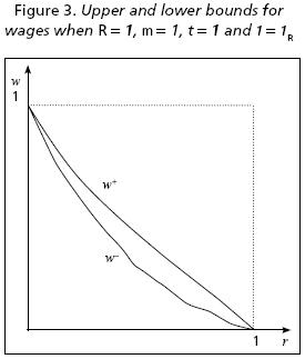
It is convenient to note that the error is zero when r = 0 or r = R. Therefore, it may be as small as desired if the levels of r being considered are close enough to any of these values. Moreover, the error diminishes as t increases. Figures 2 and 3 show the graphs of the last three formulas, respectively, when t = 0 and t = 1, with R = 1 and vector l = (¼, ¼, ½) is determined according to (13).
FINAL REMARKS
Assuming that t = 0, it follows from equation (4.a) that when the capital stock is constant, w is a linear function of r and its graph is the straight segment S(R).
Loosely speaking, we may refer to the fact that w is a continuous function of KS saying that the wage–profit curve keeps close to a straight line if the capital stock maintains close to a constant value. In the economic literature, two sufficient conditions have been pointed out for the value of capital to be constant: a) the equality between relative prices and relative values and b) the homothetic condition of the production system. In this paper, we arrived at the definition of pairs of conditions such that given any one of them the other one is sufficient for the proximity between w(r) and S(R). Indeed, if given a couple (m*, l*) a w(r) function either contained in or near to the interval determined by (22) is considered to be close to S(R), we can establish the following conclusion:
Proposition 2. In a system of type (1), in order for the wage–profit curve to be close to S(R), it is not required for the proportion between quantities produced and consumed to be near 1 + R, neither that relative prices be close to the corresponding value proportions. Any of the following two conditions is sufficient if the other one is satisfied: α) that the system belongs to a set Cm(R) such that m is either close to or less than m* and β) that the vector l of the system is close to l*.
In relation to the value of m, the empirical relevance of the set C1(R) for which some arguments were offered in sixth section may be confirmed by the quasilinearity of the wage–profit curves reported by several empirical researches, as those by Ochoa (1989), Michl (1991), Shaikh (1997), and Tsoulfidis and Rieu (2006). Indeed, if –as argued in some of these works– the studied economies satisfy either condition a) or b) indicated above, then they belong to C1(R). On the other hand, as may be appreciated in Figures 2 and 3, if a production system belongs to C1(R) the wage–profit curve is close to S(R) if vector l is close enough to lR. Nevertheless, to verify that this last condition is satisfied in the cases just cited, empirical considerations must be developed requiring another article.
We have chosen lR to calculate the numerical examples because of its peculiar properties, particularly the relation to segment S(R) that has just been mentioned, but in order to illustrate the existence of the upper and lower bounds studied here any l ∈ S (l) could have been chosen. It also permitted to illustrate the fact that these bounds can be very close to each other, suggesting that the corresponding estimation of the functions may be used eventually in empirical researches. For instance, the estimation of w by means of (22) in the case of the example presented on seventh section yields an error smaller than 6.1% and 6.13% for any r < 20%, considering respectively t = 0 and t = 1, and the error decreases tending to zero as r tends to zero.
Finally, we may add that the approach followed here to study functions KS(r) and w(r), largely based on the contributions of the authors mentioned in the introduction, is justified by the results established. Naturally, our research covered only a few properties of these functions and in order to reach further advances, for instance concerning the degree in which changes in l affect the upper and lower bounds of the functions, more studies based either on this or in other perspectives are required.
REFERENCES
Benítez, Alberto (1986), "L'étalon dans la theorie de P. Sraffa", Cahiers d'économiepolitique, 12:131–146. [ Links ] [(1990), "La mercancía patrón en la teoría de Piero Sraffa", Lecturas de Economía, 32–33: 45–68] [ Links ].
Benítez, Alberto (1995), Desequilibrio y precios de producción, México, UAM–Siglo XXI Editores. [ Links ]
Benítez, Alberto (2009), "El pago del salario", Investigación Económica, 270: 69–96. [ Links ] [(2010) "The payment of wages", Denarius, 20: 193–219] [ Links ].
Bidard, Christian (2004), Prices, Reproduction, Scarcity, Cambridge, Cambridge University Press. [ Links ]
Gantmatcher, Felix (1966), Matrix Theory, New York, Chelsea Publishing. [ Links ]
Marx, Karl (1990), Capital, Volume I, New York, Penguin Books. [ Links ]
–––––––––– (1992), Capital, Volume II, New York, Penguin Books. [ Links ]
Michl, Thomas (1991), "Wage–profit curves in US manufactures", Cambridge Journal of Economics, 15: 271–286. [ Links ]
Morishima, Mischio (1973), Marx's Economics, Cambridge, Cambridge University Press. [ Links ]
Neuman, Joseph von (1945), "A Model of General Economic Equilibrium", Review of Economic Studies, 13: 135–145. [ Links ]
Ochoa, Eduardo (1989), "Values, prices and wage–profit curves in the us economy" Cambridge Journal of Economics, 13: 413–429. [ Links ]
Pasinetti, Luigi (1977), Lectures in the theory of production, New York, Columbia University Press. [ Links ]
Ricardo, David (2004), The works and correspondence of David Ricardo, lndianapolis, Liberty Found, lnc. [ Links ]
Shaikh, Anwar (1997), "The Empirical Strength of the Labor Theory of Value", in Bellofiori, Ricardo (ed), Marxian Economics: A Reappraisal, Vol. 2, New York, St. Martin's Press. [ Links ]
Smith, Adam (1981), An inquiry into the nature and causes of the wealth of nations, Vol. i, lndianapolis, Liberty Found, lnc. [ Links ]
Sraffa, Piero (1960), Production of commodities by means of commodities, Cambridge, Cambridge University Press. [ Links ]
Steedman, lan (1977), Marx after Sraffa, London, New Left Books. [ Links ]
Tsoulfidis, Lefteris, and Rieu, Dong Ming (2006), "Labor Values, Prices of Production, and Wage–Profit Rate Frontiers of the Korean Economy", Seoul Journal of Economics, 3: 275–295. [ Links ]
1 There is a large literature on these matters, Morishima (1973) studies the division in departments I and II and presents a bibliography on the subject. Bidard (2004) compares some aspect of the models by von Neuman and Sraffa and discusses the corresponding literature. In the last work, as well as in Pasinetti (1977) the interested reader may also find an introduction to the subject.
2 Although there is no fixed capital in the model, we use the term "capital stock" in reference to the value of the physical capital in order to distinguish it from the total amount of capital, which includes the wages advanced.
3 Apart from establishing some properties of the wage–profit curve that paper discusses the antecedents of the model. For this reason, we will only mention here that the importance of the payment date for income distribution is pointed out in Chapter 6 of Marx (1990: 278) and also that Sraffa (1960: 10) considers the two payment dates schedule as the most appropriate way to treat wages, although in contraposition Steedman (1977:21) affirms that this date has no importance at all.
4 Following Marx (1990) and Sraffa (1960) we take as given the quantities produced as well as those that are used as means of production in the different industries. In Benítez (1995) a model is presented where: a) prices are constant, b) the profit rate is the same in all industries and c) the quantities produced and consumed are determined endogenously, taking demand into account.
5 Pasinetti (1977: 134) points out that when wages are paid at the beginning of production they are not included in the classical notion of net product. Nevertheless, independently of the schedule for the payment of wages, the value of the real income is equal to the net income.
Información sobre los autores:
Alberto Benítez Sánchez. Profesor–investigador de la Universidad Autónoma Metropolitana–Iztapalapa. Obtuvo los grados de maestro en Sociología y doctor en Economía por la Université Paris x–Nanterre (Francia). Sus investigaciones se desarrollan principalmente en el campo de la teoría económica y tienen como referencia central los sistemas de ecuaciones lineales de producción. Por medio de ellos, estudia temas como las relaciones entre los precios y la distribución del ingreso, además de evaluar algunas tesis de las teorías clásicas y marxistas. El criterio que adopta es lógico–formal y tiene como objetivo relevante destacar los aspectos acumulativos del trabajo científico, lo que le condujo a proponer en su libro Desequilibrio y precios de producción una síntesis de las teorías mencionadas con algunos desarrollos de las teorías no walrasianas. Ha publicado cerca de treinta textos en revistas y libros colectivos.
Alejandro Benítez Sánchez. Se graduó de ingeniero electromecánico en el Instituto Tecnológico de Tijuana y se especializó en Matemáticas en esa misma institución. Realizó una maestría en Educación en la San Diego State University y un doctorado en Educación en la Claremont Gradúate University, ambos con el patrocinio de una beca Fulbright. Ha sido catedrático de Matemáticas en diversas instituciones de educación superior mexicanas y estadunidenses. Actualmente es coordinador de la Maestría en Ingeniería Industrial en el ITT. Sus variados intereses incluyen la filosofía de la ciencia y las matemáticas aplicadas. En los últimos años se ha concentrado en el área de probabilidad y estadística, desarrollando varias distribuciones de probabilidad y trabajando en modelos lineales aplicados a la economía.

