


 nueva página del texto (beta)
 Inglés (pdf)
 Artículo en XML
 Referencias del artículo
 Enviar artículo por email
 Citado por SciELO
  Similares en
SciELO
Similares en
SciELO 
 Permalink
Introduction
Heat transfer operations are not only associated with temperature control for chemical conversions in a reactor, but in many cases they also appear during the processes of adaptation of the raw material and separation, which involve the recovery and purification of the products of interest (Fogler, 2006). For example, in the case of the sulfuric acid production by the contact method, the correct treatment of the temperature reaction remarkably influences the material costs, and the problems of air pollution (Austin, 1988).
Then, in numerous industrial applications involving heat transfer, it is extremely important to determine the rate of heat transfer for a given temperature difference. The dimensions of refrigerators, heaters, evaporators, condensers and heat exchangers depend not only on the amount of heat, but also on the rate at which this energy can be transmitted. In order to know the required flows, it is necessary to know the value of the convective heat transfer coefficient (Mobtil et al., 2018). Thus, the knowledge and understanding of heat transfer phenomena and the value of heat transfer coefficients are necessary in order to design and operate this type of industrial systems, which are relevant in the chemical processes (Majumder, 2016; Hâkansson Andreas, 2019).
In most cases, where heat transfer is involved, for various geometric configurations and flow arrangements, the coefficient is calculated by empirical and semi-empirical correlations with dimensionless groups of variables (Popiel et al., 2004, 2007). These correlations of experimental data are reported in the literature (Mills, 1995; Atmane et al., 2003). Generally, the empirical determination of the Nusselt number is used, partly because the differential equations that describe the convective heat transport model have no analytical solution, or only have it in basic cases. Another limitation of these correlations is that they rarely provide exact values for the convective coefficients, since they ignore a wide variety of conditions that depend on the type of fluid, thus considerable mistakes can be made (Blair, 1983).
Therefore, it is of great interest to explore the possibility of calculate heat transfer coefficient monitoring thermal conditions. Carson et al. (2004) measured the apparent heat transfer coefficients within a convection oven using four different methods: back-calculation from transient temperature data, heat flux sensors, the mass-loss rate, and a psychrometric method. The authors report that the most common method for determining heat transfer coefficients in convection ovens appears to be the ''transient temperature measurement'' method. This method involves fitting a mathematical model to transient temperature vs. time data and back-calculating the average the heat transfer coefficient. Additionally, Santos et al. (2017) performed transient heat transfer experiments measuring time-temperature histories and applying the finite element method to calculate the surface heat transfer coefficients in plastic cylinders of different diameters, immersed in dry ice-ethanol cooling. Ingason and Wickstrom (2007) showed that incident radiant heat flux can be obtained indirectly from plate thermometer measurements. In several applications of cooling in cylindrical geometries, the transient state of heat transfer has been studied using numerical analysis with a 3D model and simulating with Fluid Dynamics (CFD), as in the case of Ituna-Yudonago et al. (2019).
In laboratory experiments, the inaccuracy, uncertainty or data variability must be taken into account to represent the available information. The most commonly used method for estimating the uncertainty in -values is performing repeated measurements under the same conditions and use the standard deviation of the individual estimates. However, this traditional procedure will not describe the total uncertainty associated with the quantification of convective heat transfer coefficients (Hâkansson Andreas, 2019). In this case, representation of data in interval form or variation range is more appropriate. Interval-valued data (IVD) are adequate to deal with imprecise data resulting from repeated measures, bounds of the set of possible values of the item or variation range of a variable through time (Domingues et al., 2010). The proposed method can also decrease the demand on the sample number of measurement data in comparison with the classical probabilistic method (Wang et al., 2014).
This paper presents a practice of an experiment with a mercury-filled glass thermometer to determine the heat coefficient transfer by natural convection. The bulb thermometer is an available instrument in many laboratories, and could be used to calculate indirectly the heat transfer coefficient on a surface, by measuring temperature changes in transient state until thermal equilibrium is reached. The temperature data reported in this article are presented as interval-valued data, which implies using a modified least squares method to solve the proposed models.
The contribution presented here can serve as a basis for the structuring and implementation of an own laboratory guide for the learning of transport phenomena, in this case of heat, from a theoretical-practical approach. Further specifications for the approach of a more detailed methodology to carry out this experience in the laboratory can be evidenced in Chapter Sixth (entitled "Practice: Coefficient of Heat Transfer by Free Convection around a Cylinder") of the work Experimental Determination and Prediction of the Coefficient of Heat Transfer Around the Bulb of a Glass Thermometer, previously developed by the authors(1) (Mayorga Betancourt, 2010).
Materials and methods
The determination of a natural convective heat transfer coefficient around the bulb thermometer, which is cooled, was carried out in three steps: (1) experiment design and data recording, (2) construction of mathematical models and determination of the heat transfer coefficient, and (3) verification and validation of the models.
Step1. Experiment design and data recording
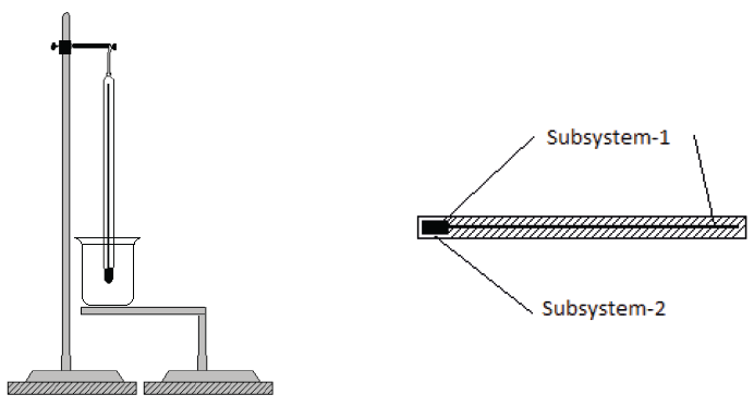
The experiment was the cooling of a bulb thermometer in free convection, oriented vertically. The precision glass thermometer was located vertically, as shown in Figure 1a. The bulb was heated with a flame until the capillary of the thermometer achieved the maximum allowable of the temperature scale. Then, the flame is removed, and a vessel is quickly placed under the thermometer, so that the bulb of the thermometer is submerged inside the vessel. The container minimizes external disturbances that could induce air currents surrounding the bulb, guaranteeing free convection. When the meniscus of the capillary column begins to descend, data temperatures were recorded in interval form as a function of time.
Step2. Construction of mathematical model and determination of the heat transfer coefficient
Two models are proposed for the experiment described. Model-I considers subsystem-1 formed by the bulb and the capillary column of the mercury thermometer, see Figure 1b. Model-II considers subsystem-1 described previously and subsystem-2 formed by the glass container holding de mercury.
The following restrictions are assumed in the construction of the models:
The bulb is the place where heat is transferred: The heat transfer in the glass container surrounding the capillary column is negligible, because it is thick enough.
Heat spreads instantaneously in the thermometric fluid, thus the capillary mercury column and the bulb have the same temperature.
Mercury does not wet the glass wall.
There is no condensation of thermometric fluid vapors on the walls of the capillary column of the thermometer.
The two subsystems that transfer heat are considered with a concentrated capacity, Bi < 0.1, thus there is no spatial temperature distribution.
After obtaining the analytical solution of the proposed models, the least squares method was applied in order to calculate the coefficient in function of experimental data. Considering that the data was interval-valued, the expression originated from the least squares method is taken as an objective function, and then minimized to obtain hlow and hupp As a result, an inequality equation is obtained to establish the variation range of the heat transfer coefficient.
Results
Measurements
Table 1 shows the main bulb thermometer specifications, and Table 2 lists the experimental conditions.
Table 1 Specifications of the mercury-filled glass thermometer.
| Name | Liquid in glass thermometer |
|---|---|
| Range, ºC | 10-35 |
| Subdivisions, °C | 0.02 |
| Long lines every, °C | 0.1 |
| Number every, °C | 0.2 |
| Maximum scale error, °C | 0.10 |
| Total length, mm | 588.50 |
| External diameter of the column, mm | 7.38 |
| Inner diameter of bulb, mm | 4.43 |
| Bulb length, L, mm | 45.3 |
| Specific heat at constant pressure of mercury, Cp, J kg-1 K-1 | 139.3(2) |
| Specific heat at constant pressure of the glass, CpV , kg-1 K-1 | 800(3) |
| M, kg | 0.00948 |
| Mv, kg | 0.00339 |
Table 2 Experiment conditions.
| T0,L (°C) | T0,U (°C) | Tƒ (°C) | TV,L,ƒ (°C) | TV,U,ƒ (°C) | tƒ (s) |
|---|---|---|---|---|---|
| 30.20 | 30.30 | 20.00 | 21.50 | 21.60 | 1135.75 |
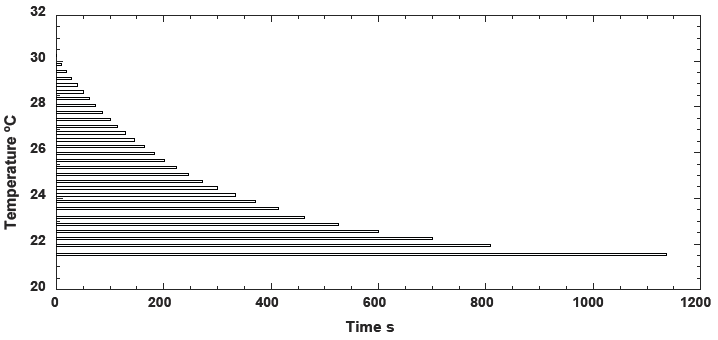
As experiment result, 30 temperature measurements in interval form were obtained and reported graphically as a function of time (Figure 2). The temperature is plotted with the interval-bar, which facilitates the reading of the temperature interval for the corresponding time. For example, in time of 1135.75 seconds, the temperature is between 21.5 and 21.6 Celsius degrees, 21.5 < T < 21.6 °C.
Model construction and solution
The main heat transfer model in the bulb thermometer was built based on the energy balance in the subsystems. Eq. (1) express the energy balance in the subsystem-1: the change in the internal energy per unit time is equal to the convective heat flow coming out of the bulb. Eq. (2) is the energy balance in the sub-system-2: the change in the internal energy per unit time of the container is equal to the heat flow coming from the bulb minus the heat flow of the container toward the environment.
with the initial condition in t = 0 , T = T0 and TV = T0.
For determining the convective heat transfer coefficient around the bulb of the thermometer, two models were constructed, and the solution was validated with the experimental data.
Solution of Model-I:
This model considers that the bulb and the glass container have the same temperature T = TV and that the heat transfer coefficients h and h∞ are equal and constant. In this case, the model-I is reduced to Eq.(3), and the analytical solution is shown in Eq. (4):
In order to determine the coefficient in terms of experimental data, the least squares method was applied to Eq. (4) in order to obtain Eq. (5):
If the data were taken in a punctual manner, it would be enough to apply Eq. (5) to determine the heat transfer coefficient. However, the experimental temperature data are in interval-valued form. Then, a double optimization strategy is required to determine the coefficient in interval form, as in Eq. (6).
Therefore, Eq. (5) becomes an objective function to minimize with the intention of determining hlow and hupp. The minimum convective coefficient h for the lower values is shown in Eq. (7).
Likewise, the coefficient for higher temperature values is showning in Eq. (8):
Therefore, the inequality expressed in Eq. (9) allows to determine de coefficient with interval form.
By programming inequality (9) with the experimental data from Figure 2, and considering the initial condition data reported in Table 2, the heat coefficient is obtained between 8.96 and 9.31 W m-2 K-1, thus h = 9.15±0.15 W m-2 K-1.
Solution of Model-II
Model-II considers the two subsystems and suppose that heat transfer coefficients both h and h∞ are equal and constant. Therefore, by solving simultaneous differential equations, represented by Eqs. (1) and (2), they are reduced to a second order differential equation with a single variable, as in Eq. (10):
with a, b, c, respectively:
The conditions TV to are:
With the two previous conditions, the solution of Eq. (10) is:
The parameters u,w,p and q are:
Since the data have been reported in the interval form, the summation to be minimized with the least squares method must also be given in the interval form as:
where Slower is the lowest value of the summation and Supper is the highest value of the summation.
Or it can be:
Applying the least squares method with the experimental data corresponding to the lowest temperatures of the interval, in this case (TVL)k, the left member of the inequality (13) is:
The numerical determination of coefficient that minimizes Eq. (14) for experimental data is: hlow = 6.10 W m-2 K-1.
Applying the least squares method with the experimental data corresponding to the highest temperatures of the interval, in this case (TVU)k, the right member of the inequality (13) is:
The numerical determination of coefficient h that minimizes Eq. (15) is: hupp = 6.29 W nr-2 K-1, whereby 6.10 < h <6.29 W m-2 K-1, that is, h = 6.2±0.1 W m-2 K-1. The heat coefficients calculated in this way included the propagation of errors due to recording error of the experimental data.
Model validation
Validation of Model-I
By expressing the glass container temperature (TV) in Eq. (4), Eq. (16) can be obtained and knowing the variation intervals of the heat transfer coefficient hlow < h < hupp and the interval of temperature variation TOL < T < TOU, TV,low and TV,upp can be determined according to Eq. (17).
The temperatures calculated with the Eq. (17) and using the Script 1 (Figure 3a) in Matlab®, then these are represented in Figure 3b with the interval-bar and the experimental data. It can be appreciated that almost all interval bars in experimental data are outside the interval-bar given by adjusted data, which means that model-I does not fit the experimental data. However, it does show the same trend as the experimental data. That is why a second model (model-II) is used.
Validation of Model-II
With the solution of model-II, Eq. (12) and the respective combination of variables, TVL and TVU are obtained in Eqs. (18) and (19), respectively:
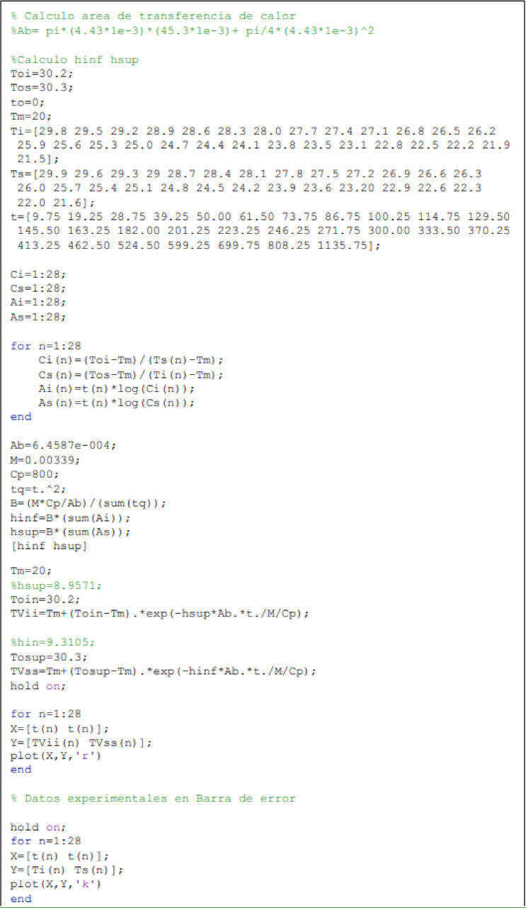
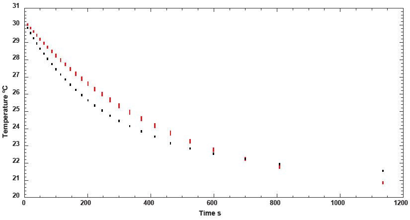
The calculated data from Eqs. (18) and (19) using Script 2 of Matlab® (Figure 4a) are plotted in Figure 4b with interval-bars, and compared with the experimental data.
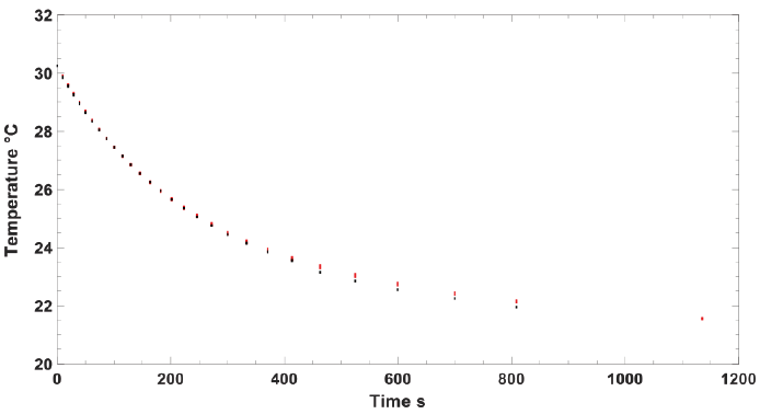
Figure 4 Model-II: (up) 4a - Script 2. (down). 4b -Calculated temperature with model-II, compared with experimental data | : Red interval-bar of adjusted data and | : Black interval-bar of experimental.
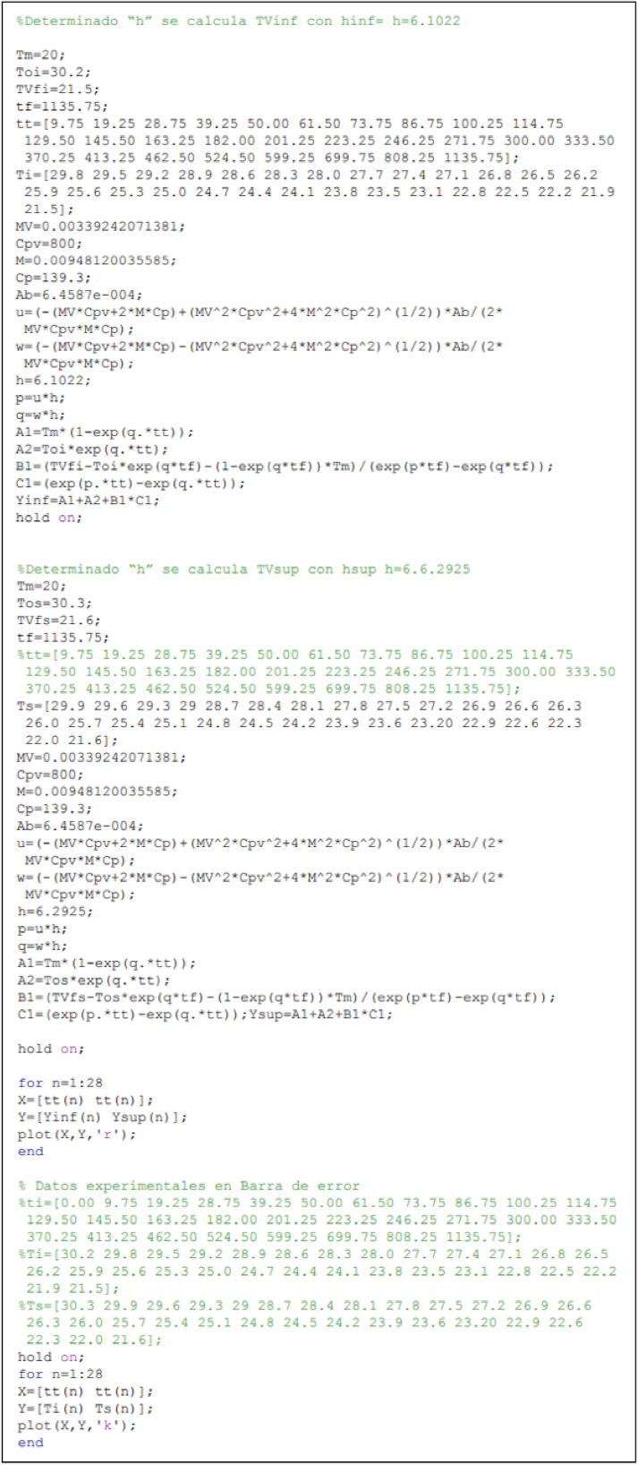
Figure 4 shows the results of model-II together with the experimental data represented with the interval-bar. This shows that most of the interval-bars of the experimental data overlap with the interval-bars adjusted by the model. This allows to conclude that Model-II is the one that best fits the experimental data for cooling of bulb thermometer in a vertical position.
Conclusions
This document describes a laboratory practice that can be implemented for the determination of the heat transfer convective coefficient. Two models were generated in transient flow to calculate the heat transfer coefficient by natural convection of mercury in the thermometer bulb, due to the descent of meniscus in the capillary mercury column in a glass thermometer. The respective analytical solutions were developed, together with the experimental data and the modified least squares method to work with data read in interval form. This allowed to measure indirectly the heat transfer coefficient in the interval form.
The first solution (Model-I) considers the temperature of the mercury bulb equal to the temperature of the glass container, while in the second solution (Model-II), this restriction was not considered. The experimentally determined coefficients values were: h = 9.15±0.15 W m-2 K-1 for Model-I and h = 6.2±0.1 W m-2 K-1 for Model-II. The two analytical solutions with their respective coefficients measured indirectly were used to predict the temperature evolution in the bulb thermometer and compare it with the experimental data. Data predicted by the restricted model-I have the same tendency as experimental data, although no good quantitative fit was evidenced. In contrast, the coefficient calculated with the unrestricted model-II showed greater quantitative coincidence between calculated and experimental temperatures.
The data measured in interval form allows taking into account the inaccuracy and uncertainty of the temperature information by the correct determination of the convective heat transfer coefficient.
Nomenclature
| Ab | Heat transfer area (m2) |
| Bi | Biot Number |
| CP | Specific heat at constant pressure (J Kg-1 K-1) |
| CPV | Specific heat at constant pressure in glass container holding mercury (JKg-1 K-1) |
| h | Convective heat transfer coefficient in the thermometer bulb (Wm-2 K-1) |
| h∞ | Convective heat transfer coefficient of the air surrounding the glass container (Wm-2 K-1) |
| hlow | Lower value of convective heat transfer coefficient in the thermometer bulb (W m-2 K-1) |
| hupp | Upper value of convective heat transfer coefficient in the thermometer bulb (W m-2 K-1) |
| M | Mercury mass in the bulb of the thermometer (kg) |
| MV | Mass of the glass container holding mercury (kg) |
| K | Indices |
| T | Mercury temperature of thermometer (K or °C) |
| Tƒ | Equilibrium temperature in the medium surrounding the thermometer bulb (K or °C) |
| T0 | Initial temperature in the medium surrounding the thermometer bulb (K or °C) |
| TV | Temperature of the glass container holding mercury (K or °C) |
| T0L | Lower value of initial temperature (K or °C) |
| T0U | Upper value of initial temperature (K or °C) |
| TV,low | Lower temperature of glass container holding mercury, calculated (K or °C) |
| TV,upp | Upper temperature of glass container holding mercury, calculated (K or °C) |
| TVL | Lower temperature of glass container holding mercury, experimental (K or °C) |
| TVU | Upper temperature of glass container holding mercury, experimental (K or °C) |
| TVLf | Final lower temperature of glass container holding mercury, experimental (K or °C) |
| TV,U,f | Final upper temperature of glass container holding mercury, experimental (K or °C) |
| t | Time, (s) |
| tf | Time corresponding to the equilibrium temperature (s) |

