


Serviços Personalizados
Journal
Artigo
 texto em
  Inglês (pdf)
 Artigo em XML
 Referências do artigo
 Enviar este artigo por email
Indicadores
-
 Citado por SciELO
 -
 Acessos
Links relacionados
-
 Similares em
SciELO
Similares em
SciELO
Compartilhar

 Permalink
Frontera norte
versão On-line ISSN 2594-0260versão impressa ISSN 0187-7372
Frontera norte vol.34 México Jan./Dez. 2022 Epub 10-Fev-2023
https://doi.org/10.33679/rfn.v1i1.2287
Articles
Price Fluctuations and the Demand for Gasoline in the Mexican Northern Border

1Tecnológico de Monterrey, México, jaibarra@tec.mx
2Investigadora independiente, México, lksotres@yahoo.com.mx
The objective of the article is to estimate the price elasticity of the demand for gasoline in Mexico’s Northern border based on applying monthly data of Mexican regions from 1997 to 2015. The results reveal that the demand for gasoline at the border is less inelastic than inland. A database is provided that includes more observations and regional economic variables compared to previous studies. It is concluded that beyond the economic effects of gasoline-related tourism, the competition faced by gas stations on the Northern border influences the price elasticity of demand. This confirms the importance of gasoline tourism in this region of Mexico, as has been recognized by federal and municipal authorities.
Keywords: demand for gasoline; price regulation; Northern border region; Mexico
El objetivo del artículo es estimar la elasticidad precio de la demanda de gasolina en la región frontera norte de México, a partir del empleo de un panel de datos mensuales de las regiones mexicanas que abarca de 1997 a 2015. Los resultados revelan que la demanda de gasolina en la frontera es menos inelástica que en el interior del país. Se aporta el uso de una base de datos que incluye un mayor número de observaciones y variables económicas regionales en comparación con estudios anteriores. Se concluye que más allá de los efectos económicos que propicia el turismo asociado a la gasolina, la competencia que enfrenta el sector en la frontera norte influye en la elasticidad precio de la demanda. Esto confirma la importancia que tiene el turismo de gasolina en dicha región de México, tal como ha sido reconocido por las autoridades federales y municipales.
Palabras clave: demanda de gasolina; regulación de precios; región frontera norte; México
INTRODUCTION
The existence of substitutes in consumption is one of the determinants of the price elasticity of demand of a product. All things being equal, the demand for a product that has substitutes is generally more elastic to changes in its price. In the case of cross-border purchases of gasoline, Moshiri (2020) and Ghoddusi, Rafizadeh, and Rahmati (2018) document that the provinces near the border in Iran, which have lower prices than those of neighboring countries, have higher price elasticity due to fuel smuggling. Similarly, Banfi, Filippini and Hunt (2005) find that their estimates of the price elasticity of demand at service stations located on the Swiss border are higher than those in the inland regions of the country. This phenomenon has also been documented in Mexico. Ibarra Salazar and Sotres Cervantes (2008) found that demand is more elastic in the Northern border region than in the rest of the country.
The objective of this paper is to estimate the price elasticity of gasoline demand in the Northern border region and compare it with that in the interior of the country, using monthly data from 1997 to 2015. Unlike the study by Ibarra Salazar and Sotres Cervantes (2008), this research uses a larger data set and considers regional economic variables to include them as determinants of gasoline demand.
This study captures the difference in price elasticity in service stations that face a dissimilar regional market as compared from those located in the interior of the country,3 when gasoline prices were regulated by the fiscal authorities in Mexico, that is, until 2015.
The results confirm the central hypothesis, and the findings in other border regions of the world: the demand in the Northern border is less inelastic than in the interior of the country and this persists in different periods. The existence of an alternative regional market with another structure and price setting mechanism, in addition to fluctuations in the MXN-USD exchange rate, effectively modify the price-quantity relationship in the borderland gasoline market.
This reality has important implications for public policy in Mexico. To illustrate, if the regulatory policy in the border region were the same as in the rest of the country, and if the price of gasoline in the Northern border of Mexico were higher than that in the southern border of the United States, then from the economic standpoint, a reduction in sales and employment in the fuel industry would be expected, and this effect could be extended to other markets, especially the commercial sector, as mentioned by Ayala Gaytán and Gutiérrez González (2004). In such case, and from the fiscal perspective, a lower excise (IEPS) and value added (IVA) tax collection would be expected in the Mexican side gasoline market. This reduction in federal tax collection would have the potential to reduce the amount of transfers received by states and municipalities throughout the country, as pointed out by Ibarra Salazar and Sotres Cervantes (2008). There may also be an environmental impact in the southern border of the United States if a considerable influx of cars, due to the so-called fiscal tourism, is observed. The border crossing waiting time is also a factor that can influence the increase in economic costs.
The evolution of the demand for gasoline, and a discussion on retaled demand studies for this fuel in the Northern border region of Mexico are presented below. After that, the methodology used in this study, its results and conclusions are presented.
Evolution of Gasoline Demand
According to sales data from Pemex (Petróleos Mexicanos) agencies during the period under study, the average monthly sales volume of gasoline (Magna and Premium) in the Northern border region was 276 million liters (ml), while in the interior of the country it was 3,015 ml. Border sales represented an average of 8.4% of total sales in Mexico (Mexican Secretariat of Energy, 2021).
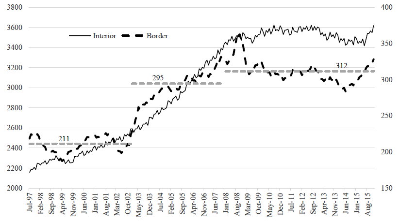
Graph 1 shows the gasoline sales smoothed series, using six-month moving averages, of the Northern border and the rest of the country. From February 1995 to December 2002, the only difference between prices in both regions was the VAT, which was 10% in the border region. From January 1997 to November 2002, the price of gasoline in the Northern border region was not equal to that of the southern of the United States (U.S.). The nominal price at the border was 2.97 MXN and the monthly sales volume was 207 ml, while in November 2002 the price rose to 5.93 MXN and the monthly sales volume was 206 ml. In this period, the monthly average of the volume of sales in that region behaved relatively stable, varying between 170 and 240 ml.
Source: Own elaboration based on the Mexican Secretariat of Energy (2021).
Graph 1. Volume of gasoline sales in the Northern border region and in the interior of Mexico (from June 1997 to December 2015) Note: The sales volume in the Northern border region is measured on the right axis.
From January 2003 to December 2007, a clear positive trend is observed in the gasoline sales volume both in the interior of the country and in the Northern border region. With the prices of this fuel on the Mexican border aligned to those on the southern border of the United States, the sales volume went from 252 ml in January 2003 to 342 ml in December 2007: a 35.8% growth. The monthly average volume in such a period was 295 ml.
From January 2008 to December 2015, a policy to adjust the price of gasoline was implemented in Mexico in order to eliminate the subsidy that was granted through the IEPS, since, given the price increase of oil and the mechanics of gasoline pricing, the IEPS was negative. When the price of oil dropped, in the first quarter of 2014, the subsidy disappeared. For this reason, the nominal price of gasoline in 2015 did not change. In that period, in which the price had controlled monthly adjustments, the average monthly gasoline sales volume in the border region was 312 ml. Graph 1 shows that, during this period, the sales volume had a negative trend.
Literature
Despite of being a central issue in price and fiscal policies in the Mexican gasoline market, the analysis of the demand for this fuel in the Northern border region of Mexico has not received the attention it deserves. From the 1990s, and even before the liberalization of prices in 2017, based on the evolution of the international price of oil and the MXN-USD exchange rate, gasoline prices in the Northern border had periods of homologation with southern U.S. prices as well as periods of prices aligned to those of the interior of the country. In terms of the fiscal policy, VAT rates on gasoline in the Northern border region have been set below the national rate. Indeed, the gasoline market in the Northern border of Mexico has been the object of special treatment in terms of the regulated pricing policy and of the fiscal policy. However, scholars of that sector in this region have not responded accordingly to its relevance: there are only four published articles on the demand for gasoline in the Northern border region of Mexico (Fullerton et al., 2012; Ibarra Salazar & Sotres Cervantes, 2008; Ayala Gaytán & Gutiérrez González, 2004; Haro López & Ibarrola Pérez, 1999).
The works by Ayala Gaytán and Gutiérrez González (2004), and Haro López and Ibarrola Pérez (1999) use monthly data from the border areas that were defined in 1991 to implement a homologation policy with U.S. prices.4 As a matter of fact, from 1991 to 1995, the prices of this fuel on the Northern border of Mexico were equal to those that prevailed on the southern border of the United States in the six zones that were defined for this purpose. The depreciation of the Mexican peso led to the end of this policy at the beginning of 1995 and, as of February of that year, prices were uniform throughout Mexico, with a VAT rate of 10% on the Northern border. The evolution of the price of oil, which led to a reduction in the price of gasoline in the U.S., contrasted with the continuous increase in prices in Mexico and, as a result, as of 1997, prices in the U.S. southern border were lower than those in Mexico (Ibarra Salazar & Sotres Cervantes, 2008; Ayala Gaytán & Gutiérrez González, 2004; Haro López & Ibarrola Pérez, 1999). Faced with this prevailing situation, towards the end of the 1990s, the works by Ayala Gaytán and Gutiérrez González (2004) and Haro López and Ibarrola Pérez (1999) analyze the demand to observe the effects of the homologation of gasoline prices in the U.S.-Mexico border, a measure that was eventually implemented as of November 2002 (Ibarra Salazar & Sotres Cervantes, 2008). Thus, Ayala Gaytán and Gutiérrez González (2004) estimated that the homologation of prices in 2000 would cause the demand to be 3 500 million liters, which compared to the 2 579 million liters sold in that year, meant that uniform prices would have an effect of a 36% increase in gasoline sales.
The changing pricing policy towards the Northern border in those years also motivated the study by Haro López and Ibarrola Pérez (1999), although the main issue in this case is the fiscal effect. The estimation of elasticities is an important element to determine the effect of price and fiscal policy on the collection of IEPS and VAT.
In a different context, the study by Fullerton et al. (2012) analyzes the demand for gasoline in Ciudad Juárez, Chihuahua, considering monthly data from January 2000 to December 2009. Ibarra Salazar and Sotres Cervantes (2008), although studying this same topic, use a monthly panel data set of the Mexican states, since their purpose is to compare the sensitivity of demand to changes in its price in the Northern border and in the non-border region.
The article by Fullerton et al. (2012) applies time series estimation techniques (Autoregressive Integrated Moving Average [ARIMA] model transfer functions) to study the dynamics of demand in one of the most important cities of the Northern border region of Mexico. Dynamic considerations in the demand model also appear in the work of Ayala Gaytán and Gutiérrez González (2004). To capture this aspect, they include binary variables to control for seasonality and a one-period sales lag. With this structure it was possible to estimate the difference between the short- and long-run elasticities with respect to the independent variables.
Gasoline tourism causes a series of consequences in the borderland markets of this fuel. A documented case is that of Luxembourg, where less taxes are charged as compared to neighboring countries (Germany, France and Belgium). In this country, the so-called tank tourism represents an important source of fiscal revenue for the government, but also an environmental problem (Luxembourg Times, 2014). It was estimated that in 2016 77% of the demand came from non- residents (Toussaint, 2019). The direct consequences of this phenomenon can be observed in the gasoline market (sales, employment, among other variables), in the commercial sector in general, in tax collection, in environmental pollution (due to the increase in traffic and congestion), and in the welfare of consumers (Kennedy, Lyons, Morgenroth, & Walsh, 2017; Leal, López-Laborda y Rodrigo, 2010). The effect of gasoline tourism in the commercial sector is analyzed in Ayala Gaytán and Gutiérrez González (2004), while the fiscal consequences, although not in tax collection, but in the recognition of the consequences beyond the border region, have been considered in Ibarra Salazar and Sotres Cervantes (2008). Thus, the price and fiscal policy towards the border affects the federal tax collection (VAT & IEPS) and, therefore, also influences the amount of transfers that are distributed among all Mexican states and municipalities. Due to this, Ibarra Salazar and Sotres Cervantes (2008) recognize that this phenomenon in the Northern border has consequences in the fiscal revenue of each and every one of the subnational governments in the country.
The direct effects of gasoline tourism in the U.S.-Mexico border, as well as the indirect ones on the commercial sector, have not been measured; even less have been measured, the environmental consequences as a result of this phenomenon. The fiscal consequences, although identified, have not been estimated either.
When using regional data, the economic variables of control can represent a complex challenge. In the case of gasoline demand studies with a regional data structure and monthly frequency, there is a significant limitation in having variables that allow controlling for economic and socio- demographic characteristics (Ghoddusi, Morovati, & Rafizadeh, 2019). The economic environment is included in various ways in studies of demand in the border region. The work of Fullerton et al. (2012) includes formal employment in Ciudad Juárez; Haro López and Ibarrola Pérez (1999), based on data from the state Gross Domestic Product (GDP), created a per capita income figure for the different border areas, and also used the retail sales index of the commercial sector, which is available for particular cities. Ayala Gaytán and Gutiérrez González (2004) include employees and wages related to the maquiladora industry. Ibarra Salazar and Sotres Cervantes (2008) include a series of economic variables to assess the consistency of their results: some that are only available on a national scale (physical volume index of industrial activity and the coincident index), and some that at the time, were available on a regional scale (net retail sales index of commercial establishments, general rate of open unemployment, index of physical volume of production of the manufacturing industry, as well as index of physical volume of electricity generation and distribution).
Regarding the results, Ayala Gaytán and Gutiérrez González (2004) find that the relative price elasticity of short-term gasoline demand ranges from -0.104 in zone IB (Mexicali) to -0.41 in zone IV (Coahuila); while the long-run elasticity ranges from -0.131 in zone IA (Baja California) to - 1.696 in zone IV (Coahuila).
The results of Haro López and Ibarrola Pérez (1999) indicate that price elasticity ranges from - 0.153 in zone 1B (Mexicali) to -0.608 in zone IV (Coahuila). In the Northern border region, the estimated elasticity is -0.415. They also estimate the price elasticity for the border states: for Baja California their estimate is -0.156; for Sonora, -0.309; for Chihuahua, -0.367; for Coahuila, -0.407; for Nuevo León, -0.092, and for Tamaulipas, -0.543.
Fullerton et al. (2012) estimate that the price elasticity of demand for gasoline in Ciudad Juárez is -0.57. Ibarra Salazar and Sotres Cervantes (2008) show evidence that the demand for gasoline is less inelastic in the Northern border than in the interior of the country. According to the different specifications, in which they include different economic variables, they estimate that the elasticity in the Northern border region varies between -0.67 and -1.57, while for the rest of the country it ranges from -0.15 to -1.06.
Table 1 shows in a comparative way some of the characteristics of the studies described.
Table 1. Studies on gasoline demand about the Northern border region of Mexico
| Borderland | The present study | Ibarra Salazar and Sotres Cervantes (2008) |
Ayala Gaytán and Gutiérrez González (2004) |
Haro López and Ibarrola Pérez (1999) |
|---|---|---|---|---|
| Data | Monthly data
panel of the Mexican states, from January 1997 to December 2015. |
Monthly data
panel of the Mexican states, from January 1997 to December 2003. |
Monthly time
series of the border areas, from January 1993 to May 2001. |
Monthly time
series of the border areas, from January 1995 to July 1999. |
| Independent variables | Price,
economic, number of registered cars in circulation. Binary variables to identify the border region. |
Price,
economic, number of registered cars in circulation. Binary variables to identify the border region. |
Relative
price, economic, gasoline sales with one month lag. Binary variables for seasonality. |
Relative prices, economic. |
| Estimation method | OLS with
Newey-West correction. |
OLS with
Newey-West correction. |
OLS | OLS |
| Estimated price elasticities | ||||
| Zone IA (B) | -0.35 | -0.71 | -0.119 | -0.296 |
| Zone IB Mexicali (B) | ND | ND | -0.104 | -0.112 |
| Zone II (S) | -1.28 | -1.93 | -0.238 | ND |
| Zone III (CH) | -0.69 | -1.16 | -0.107 | -0.438 |
| Zone IV (C) | ND | ND | -0.410 | -0.639 |
| Zone V (T) | -0.62 | -1.22 | -0.240 | -0.505 |
Source: Own elaboration based on data from the referred articles.
Note: Footnote 4 shows the municipalities included in each zone. This study and that of Ibarra Salazar and Sotres Cervantes (2008) use data from the Pemex agencies that are located in the cities of the Northern border. The works of Ayala Gaytán and Gutiérrez González (2004) and Haro López and Ibarrola Pérez (1999) are based on data from the border areas referred to in the same note. B=Baja California, S=Sonora, CH=Chihuahua, C=Coahuila and T=Tamaulipas.
METHODOLOGY
As Ghoddusi et al. (2019) note, the studies on the aggregate demand for gasoline, in addition to price, include the consumers’ income and the number of vehicles as independent variables. The price and consumers’ income are considered, par excellence, the determinants of product demand. Since the demand for gasoline is considered to be derived from the demand for automobile transport, it is a reduced form of it, and as such an input of the demand for transport would include the number of vehicles (Dahl, 1979; Archibald & Gillingham, 1980). For convenience’s sake, when the objective is to estimate elasticities, demand is specified in log-linear form since the parameters represent elasticities. Our reference model is:
where G is the demand for gasoline, P is the price of gasoline per unit, Y is the consumers’ income, V is the number of registered vehicles, and ε is the error term. The observation unit of each variable has two dimensions: time and region. The first one has a monthly frequency that goes from January 1997 to December 2015, while the second one corresponds to the cross sections, which are the federal entities in which there are sales superintendencies, sales agencies, warehouses, land and maritime terminals of Pemex, and the border areas in which these points of sale associated with their service stations could be identified.
The period considered in this study ends in 2015, the last year in which the Mexican tax authority set gasoline prices in Mexico. Two reasons justify the use of data up until that period: the first is related to the availability of regional prices; the second, with the modification in the regulation of prices towards the sector. As discussed later, 2016 was a transition year before the liberalization of prices in 2017, and as of 2016, the mechanics in setting the IEPS were different. Although regional gasoline sales data can be accessed after 2015, regional gasoline price data is not available after that year, as required to estimate the models specified in this work. With the deregulation of the gasoline industry, prices are no longer uniform in both the interior of the country and the Northern border region. In addition to this, we believe that this structural change in price regulation on a national scale deserves to be studied to determine if it resulted in changes in the price elasticity of gasoline.
Making this regionalization of gasoline demand, the parameter α 1 in the equation (1) provides an estimate of the price elasticity of gasoline for Mexico. This value can be contrasted with existing estimates of elasticity at a national scale (Ortega Díaz & Medlock, 2021; Sánchez, Islas, & Sheinbaum, 2015; Reyes, Escalante, & Matas, 2010; Crôtte, Noland, & Graham, 2010; Galindo, 2005; Eskeland, & Feyzioğlu, 1997; Berndt & Botero, 1985), even though the data structure and estimation methods may differ from those used in this work. The parameter α 2 represents the income elasticity and α 3 the elasticity of gasoline demand with respect to the number of registered vehicles.
In the second model, we incorporate a binary variable to indicate which observations correspond to the border region (DF). This variable takes the value of 1 for all the months that we have in our database, if the observation refers to the Northern border region. These include four cross sections for the border areas of Baja California, Sonora, Chihuahua and Tamaulipas. By multiplying the natural logarithm of the gasoline price, the parameter αF in equation (2) captures the difference between the price elasticity of demand in the Northern border region as compared to that of the rest of the country.
In equation (2), the price elasticity of demand for the interior of the country is α1, while the elasticity of the Northern border region, when DF = 1, is α1 + αF. Our hypothesis is that the parameter αF is negative and statistically different from zero. This would make the absolute value of the elasticity of demand in the Northern border region larger, and therefore demand in the Northern border region less inelastic (or more elastic) with respect to price as compared to the demand in the rest of the country. The αF parameter captures the Northern border effect on the price elasticity of gasoline demand. The statistical significance test on this parameter allows us to assess the evidence on the Northern border effect. Taking the value of the elasticity in the rest of the country, this effect provides the change in the price elasticity of demand for the Northern border region of Mexico.
From the study by Ibarra Salazar and Sotres Cervantes (2008), which obtained data up to December 2003, it is of interest to determine if there is evidence of structural change in the gasoline market, particularly in relation to the border effect in said market. Beginning in the early 2000s, there were significant changes in the fuel pricing policy. In the Northern border region, since the last month of 2002, gasoline prices have been aligned between peer cities across the border. Due to the increase in the international price of oil, the price of gasoline on the Northern border was higher than in the rest of the country. Thus, as of May 6, prices in that region were set at the minimum level recorded on the week of April 11 to 17, 2006. According to a communication from the Mexican Ministry of Finance and Public Credit (SHCP), this implied a reduction of more than 10% concerning the prices in force on April 24 of that year. That level would be maintained until the international references fell below the announced level, and thereafter they would follow their southern U.S. reference (SHCP, 2006).
On a national scale, the administered price scheme for fuels had as a consequence that domestic prices did not follow the trend of either the oil price or the reference used to determine the IEPS on gasoline. Between January 2000 and July 2008, regular gasoline increased its price by nearly 50%, going from 4.81 to 7.21 MXN per liter, although the price of gasoline on the U.S. Gulf Coast (USGC) increased 198%, following the trend of the international price of Brent oil (Federal Commission of Economic Competition [Cofece], 2019). This trend contrasts with the one observed between January 2010 and March 2018, when the price of gasoline increased by approximately 10 MXN per liter, although between mid-June 2014 and January 2016 the price of oil fell significantly from 148.26 at 34 USD per barrel.
To maintain the uniform pricing policy nationwide, until December 2015, the monthly IEPS rate was adjusted to accommodate the reference price (USGC) and the price set by the SHCP. When the reference price was above the market price, the tax was negative, thus implying a fuel subsidy. In 2008 this situation became unsustainable as the subsidy was MXN 242 billion. To phase it out gradually, prices had monthly managed increases. This sliding policy, coupled with reductions in the price of oil since the second quarter of 2014, reversed this situation. As of 2016, the IEPS is a flat-rate tax (Cofece, 2019).
To find out if the price elasticities of the demand for gasoline in the border and non-border regions have changed, starting from model (2), we introduce a temporary binary variable. We define the variable DE, which takes the value of 1 in each cross-section observation if it corresponds to a date of period I (between January 1997 and December 2003) and takes the value of 0 if it belongs to period II (January 2004 to December 2015). The study by Ibarra Salazar and Sotres Cervantes (2008) uses data from period I. Our estimates could differ in that period due to the economic variables at the regional scale that we use in this paper. In addition to the comparison with period I, this formulation will allow us to prove whether there was a structural change in the price elasticity of demand by comparing the price elasticities in periods I and II. The model that incorporates this temporary dichotomous variable is:
In equation (3), the price elasticity of demand in the Northern border region (DF = 1) during period I (DE = 1) is α1 + αF + αE + αEF, and in period II it is α1 + αF . Thus, the hypothesis test to find out if αE + αEF = 0 will tell us if there was a change in the price elasticity of demand of the Northern border region between periods I and II. In the case of the interior of the country, the difference in the price elasticity of demand between periods is determined by the parameter αE . Now, in period I, the Northern border effect on gasoline demand is estimated by αF + αEF; while in period II it is equal to αF. It can be noted that the structure in model (3) includes the temporal dimension (period I vs period II) and the regional dimension (Northern border compared to the interior of the country), similar to that of the Difference-in-Differences models (Angrist & Pischke, 2015).
The parameter αEF is the difference in the change in the elasticity of both regions between periods I and II. Thus, that parameter is the difference between αE + αEF , the change in elasticity between periods in the Northern border region, and αE, the change in elasticity in the non-border region. It also represents the difference in elasticity between the border and non-border regions in period I (αF + αEF ) and αF , which is the contrast in elasticity between those regions in period II.
In the fourth model we focus on the differences in the price elasticity of gasoline demand between the different areas of the Northern border. We thus include binary variables that identify the different border zones (Dj):
where j = Baja California (B), Sonora (S), Chihuahua (CH) and Tamaulipas (T). The parameters αj represent the border effect of each border zone. This is so since while α1 is the price elasticity of demand within the country, α1 + αj is the elasticity of the border zone j = B, S, CH, T. The hypothesis test to determine if demand is less inelastic in each border zone consists in rejecting the null hypothesis αj = 0, in favor of the alternative hypothesis in which αj < 0, for each border region j. A matter of interest is also whether this border effect is uniform. If so, then αB = αS = αCH = αT .
To approximate the demand for gasoline (G), we use the volume of monthly internal sales of Nova, Magna and Premium gasoline made through the sales superintendencies, sales agencies, warehouses, and land and sea terminals of Pemex. These data were obtained from the Energy Information System (SIE) of the Mexican Ministry of Energy. We assigned gasoline transactions from these Pemex points of sale to the state where they are located. Since there are no agencies in Quintana Roo and Tlaxcala, these states are not included in the database. On the other hand, additional observations in the border areas of Baja California, Sonora, Chihuahua and Tamaulipas are considered. The first includes the sales superintendencies of Mexicali and Rosarito; the border zone of Sonora includes the foreign warehouse of Cananea and the sales superintendence in Nogales; the border zone of Chihuahua includes the sales superintendence of Ciudad Juárez, and the Tamaulipas border zone includes those of Nuevo Laredo and Reynosa. In this way, the data panel is made up of 34 crossed sections: 30 states and four border areas. Since there are no Pemex superintendencies in the border area of Nuevo León and Coahuila, we do not include these areas as border areas in the database.
The price of gasoline (P) is the average monthly price per liter of Nova, Magna and Premium gasoline. This variable was obtained from the Petroleum Indicators publication (National Institute of Transparency, Access to Information and Protection of Personal Data [INAI], 2021), in which the price is differentiated for the Northern border area and for the rest of the country.5 Therefore, for the 30 states, the price of gasoline from the interior of the country is taken, while for the four border areas of Baja California, Sonora, Chihuahua and Tamaulipas, the price of the Northern border is taken. It is presented in real 2018 MXN value.
The variable V refers to the number of registered cars in circulation in each state. This is yearly data and comes from the statistics of Registered Motor Vehicles in Circulation (National Institute of Statistics and Geography [Inegi], n.d.g). Due to its annual frequency, the observation is repeated for all the months of the corresponding year. An additional limitation of this variable is that it does not capture irregular vehicles or those of American residents or citizens living on the Northern border of Mexico.6
To approximate consumers’ income (Y) we take the state GDP. Like the previous variable, this variable has an annual frequency, so the same observation is repeated in all the months of a year. It was obtained from the National Accounts System of Mexico (Inegi, n.d.f) and the units are billions of MXN in real terms (2013 = 100). We used other economic indicators, which are available on monthly or quarterly basis, as control variables to capture the general economic evolution:
Index of physical volume of the manufacturing industry (MAN), available on a regional scale and quarterly basis.
Index of physical volume generation, transmission and distribution of electricity, supply of water and gas through pipelines to the final consumer (ELEC), with a quarterly frequency and available on a regional basis.
Index of industrial activity (IND), with monthly frequency and disaggregated by state.
Coincident economic activity index (ICO), with monthly frequency and on a national scale, for which it is the same in all states.
Quarterly indicator of state economic activity (ITAEE), with quarterly frequency and disaggregated by state. It is a short-run indicator that offers a general view of the states’ economy. It is integrated with the results of the National Survey of Construction Companies, the Monthly Survey of the Manufacturing Industry and the Monthly Survey of Commercial Firms.
The variables MAN, ELEC and IND are only available from January 2003, so the estimates where they are included have fewer observations (Inegi, n.d.c, d, f). We only take one economic variable at a time to estimate the different models.
Table 2 presents the description of variables and sources of information. We use 7 752 observations (228 months for 34 cross sections). The descriptive statistics and the correlation matrix are presented in Table 3.
Table 2. Description of variables and sources of information
| Variable | Description | Period | Frequency | Coverage | Source |
|---|---|---|---|---|---|
| G | Internal sales volume of Nova, Magna and Premium gasoline in liters. |
1997-2015 | Monthly | Regional |
Secretaría de
Energía, 2021 |
| P | Average price of Nova, Magna and Premium gasoline per liter (2018 MXN value). |
1997-2015 | Monthly | Regional | Inai, 2021 |
| V | Number of registered cars in circulation. |
1997-2015 | Annual | Regional | Inegi, n.f.g |
| GDP | State Gross Domestic Product, base 2013=100 (billions of 2013 MXN value). |
1997-2015 | Annual | Regional | Inegi, n.f.f |
| MAN | Physical volume of production index (2013=100). |
2003-2015 | Quarterly | Regional | Inegi, n.f.e |
| ELEC | Physical volume index of the generation, transmission and distribution of electricity, supply of water and gas through pipelines to the final consumer (2013=100). |
2003-2015 | Quarterly | Regional | Inegi, n.f.d |
| IND | Industrial production index (2013=100). |
2003-2015 | Monthly | Regional | Inegi, n.f.c |
| ICO | Coincident index of economic activity (2013=100). |
1997-2015 | Monthly | Nacional | Inegi, n.f.b |
| ITAEE | Quarterly indicator of state economic activity (2013=100). |
1997-2015 | Quarterly | Regional | Inegi, n.f.a |
| DF | Takes the value of one (1) for the border areas of Baja California, Sonora, Chihuahua and Tamaulipas, and zero in any other case. |
1997-2015 | Own elaboration |
||
| DE | Takes the value of one (1) for t=January 1997 to December 2003, and zero (0) in any other case. |
1997-2015 | Own elaboration |
||
| DB | It takes the value of one (1) for the border zone of Baja California, and zero (0) in any other case. |
1997-2015 | Own elaboration |
||
| DCH | Takes the value of one (1) for the border zone of Chihuahua, and zero (0) in any other case. |
1997-2015 | Own elaboration |
||
| DS | Takes the value of one (1) for the border area of Sonora, and zero (0) in any other case. |
1997-2015 | Own elaboration |
||
| DT | Takes the value of one
(1) for the border area of Tamaulipas, and zero (0) in any other case. |
1997-2015 | Own elaboration |
||
Source: Own elaboration based on the sources of information indicated in this table.
Table 3. Descriptive statistics and correlation matrix
| Variable | Average | Maximum | Minimum | Standard deviation |
N | ||||
|---|---|---|---|---|---|---|---|---|---|
| G | 96 729 561 | 600 000 000 | 5 059 850 | 87 399 260 | 7 752 | ||||
| P | 12.32 | 16.07 | 9.65 | 1.48 | 7 752 | ||||
| V | 560 124 | 4 626 870 | 29 793 | 664 257 | 7 752 | ||||
| GDP | 444.07 | 2 869.79 | 61.38 | 423.85 | 7 752 | ||||
| MAN | 95.67 | 131.03 | 53.47 | 12.16 | 5 304 | ||||
| ELEC | 89.45 | 340.16 | 26.64 | 22.96 | 5 304 | ||||
| IND | 94.72 | 181.01 | 48.48 | 15.08 | 5 304 | ||||
| ICO | 95.32 | 107 | 77.7 | 5.57 | 7 752 | ||||
| ITAEE | 86.93 | 148.51 | 50.49 | 13.95 | 7 752 | ||||
| G | P | V | GDP | MAN | ELEC | IND | ICO | ITAEE | |
| G | 1.0000 | ||||||||
| P | 0.1458 | 1.0000 | |||||||
| V | 0.8431 | 0.2417 | 1.0000 | ||||||
| GDP | 0.8547 | 0.1098 | 0.8662 | 1.0000 | |||||
| MAN | 0.1859 | 0.4201 | 0.1906 | 0.1740 | 1.0000 | ||||
| ELEC | -0.0092 | 0.5748 | 0.0531 | -0.0098 | 0.2402 | 1.0000 | |||
| IND | 0.0860 | 0.4176 | 0.1339 | 0.1952 | 0.5954 | 0.4026 | 1.0000 | ||
| ICO | 0.1224 | 0.7547 | 0.1899 | 0.0969 | 0.4303 | 0.4314 | 0.3931 | 1.0000 | |
| ITAEE | 0.0900 | 0.6915 | 0.1885 | 0.2041 | 0.5250 | 0.4979 | 0.8227 | 0.6165 | 1.0000 |
Source: Own elaboration based on the sources of information presented in Table 2.
Like Ibarra Salazar and Sotres Cervantes (2008), the models were estimated using Ordinary Least Squares, correcting errors through the Newey-West method. We note that the very specification of the models assumes that there are no other independent variables that could cause differences in gasoline demand between Mexican regions. To assess the robustness of our results, we estimate different regressions of each model including the different approximations of consumer’s income and the evolution of regional economies.
RESULTS
Table 4 shows the results of model 1, which does not include the identification of border areas. We can notice that, in the first five regressions, the parameters that represent the elasticities with respect to the price of gasoline (P) are negative, although in no case the parameter is statistically significant. The elasticity of demand with respect to the number of vehicles in circulation (V) is, in all cases, positive and statistically different from zero. The estimated value in this model varies between 0.57 and 0.62. In relation to the different variables that we use to approximate the consumers’ income, we can observe that the signs obtained are not uniform. The approximation we made through state GDP shows a direct relationship and the parameter is statistically significant. The estimated income elasticity in the regression is 0.08. In that same regression the estimated price elasticity of demand is -0.05. Model 1 provides us with a figure of the price elasticity of demand for gasoline on a national scale. In regression 1 of Table 4, which does not include the economic control variable, the estimate of this elasticity is -0.11.
Table 4. Results of the estimates of model 1, lnG=α0+α1lnP+α2lnY+α3lnV+ε
| Regression | 1 | 2 | 3 | 4 | 5 | 6 | 7 |
|---|---|---|---|---|---|---|---|
| Constant | 10.45 | 10.50 | 10.45 | 10.99 | 11.69 | 11.53 | 11.65 |
| (21.79)* | (21.74)* | (11.23)* | (18.35)* | (15.52)* | (6.13)* | (21.99)* | |
| ln P | -0.11 | -0.05 | -0.38 | -0.23 | -0.11 | 0.01 | 0.51 |
| (-0.51) | (-0.25) | (-1.50) | (-0.82) | (-0.43) | (0.03) | (1.98)* | |
| ln V | 0.62 | 0.57 | 0.61 | 0.61 | 0.62 | 0.62 | 0.62 |
| (26.45)* | (15.45)* | (23.04)* | (23.16)* | (23.81)* | (26.47)* | (27.25)* | |
| ln GDP | 0.08 | ||||||
| (1.90)** | |||||||
| ln MAN | 0.17 | ||||||
| (0.87) | |||||||
| ln ELEC | -0.04 | ||||||
| (-0.46) | |||||||
| ln IND | -0.28 | ||||||
| (-1.85)** | |||||||
| ln ICO | -0.30 | ||||||
| (-0.59) | |||||||
| ln ITAEE | -0.63 | ||||||
| (-5.11) | |||||||
| Adj R2 | 0.4644 | 0.4665 | 0.4261 | 0.4255 | 0.4279 | 0.4645 | *0.4717 |
| N | 7 752 | 7 752 | 5 304 | 5 304 | 5 304 | 7 752 | 7 752 |
Source: Own elaboration based on the Ordinary Least Squares method with the Newey-West correction.
Note: t-student statistics are shown in parentheses below the estimated parameters. Numbers with an asterisk
*are significant with p-value < 0.05. Numbers with two asterisks
**have significance with p-value < 0.10. Table 2 contains the description of the variables and sources of information.
The results of the estimation of model 2, which identifies the Northern border region, are shown in table 5. The parameters of the different variables that we included to control for the evolution of consumers’ income and/or regional economic activity did not turn out to be statistically different from zero, with the exception of the ITAEE, although its sign is not as expected. In addition, the sign obtained for the parameters of these variables is not consistent in the different regressions. This result is contrary to what we can see with respect to the variable that controls for the differences in registered vehicles in circulation (V). The variable parameter ln V is positive and statistically significant in all regressions. In addition to that, the estimated value of the parameter is consistent in the different regressions shown in Table 5. In regression 1 of table 5, the elasticity of gasoline demand with respect to registered vehicles is 0.69.
Table 5. Table 5. Results of the estimations of model 2, lnG=α0+α1lnP+αFDFlnP+α2lnY+α3lnV+ε
| Regression | 1 | 2 | 3 | 4 | 5 | 6 | 7 |
|---|---|---|---|---|---|---|---|
| Constant | 10.48 | 10.30 | 10.83 | 11.32 | 9.27 | 11.12 | 10.51 |
| (24.63)* | (12.94)* | (20.00)* | (17.06)* | (5.49)* | (22.86)* | (24.53)* | |
| ln P | -0.47 | -0.64 | -0.60 | -0.43 | -0.61 | -0.14 | -0.44 |
| (-2.46)* | (-2.52)* | (-2.28)* | (-1.63) | (-2.30)* | (-0.52) | (-2.24)* | |
| DF ln P | -0.35 | -0.33 | -0.33 | -0.33 | -0.35 | -0.35 | -0.35 |
| (-8.77)* | (-7.17)* | (-7.10)* | (-6.93)* | (-8.78)* | (-8.42)* | (-8.61)* | |
| ln V | 0.69 | 0.67 | 0.68 | 0.68 | 0.69 | 0.69 | 0.67 |
| (30.75)* | (27.24)* | (26.27)* | (27.49)* | (30.73)* | (31.33)* | (18.13)* | |
| ln MAN | 0.19 | ||||||
| (1.00) | |||||||
| ln ELEC | 0.04 | ||||||
| (0.45) | |||||||
| ln IND | -0.18 | ||||||
| (-1.13) | |||||||
| ln ICO | 0.34 | ||||||
| (0.74) | |||||||
| ln ITAEE | -0.33 | ||||||
| (-2.29)* | |||||||
| ln PIB | 0.04 | ||||||
| (1.11) | |||||||
| Adj R2 | 0.5743 | 0.5371 | 0.5364 | 0.5373 | 0.5745 | 0.5763 | 0.5749 |
| N | 7 752 | 5 304 | 5 304 | 5 304 | 7 752 | 7 752 | 7 752 |
| Estimated price elasticities | |||||||
| Interior of the country |
-0.47 | -0.64 | -0.60 | -0.43 | -0.61 | -0.14 | -0.44 |
| Northern border region |
-0.83 | -0.96 | -0.93 | -0.75 | -0.96 | -0.49 | -0.79 |
Source: Own elaboration based on the Ordinary Least Squares method with the Newey-West correction
Note: t-student statistics are noted in parentheses below the estimated parameters. Numbers with an asterisk
*have p-value < 0.05. Numbers with two asterisks
**have p-value < 0.10. Table 2 contains the description of the variables and sources of information.
The ln P parameter, which shows the price elasticity of demand in the non-border region, is negative and statistically different from zero in all the regressions in table 5, except regressions 4 and 6. The estimated values vary from -0.14 in regression 6, to -0.64 in regression 2. Due to the inconsistency of the results obtained concerning our approximations of consumers’ income, if we take regression 1 as representative of our results, then the estimate of the price elasticity of gasoline demand in the interior of the country would be -0.47.
The results also indicate that the estimated border effect in the different regressions ranges from -0.33 to -0.35 and is statistically significant in all cases. This means that demand is less inelastic in the Northern border region than in the interior of the country. Given an adjustment in the price of gasoline, say by 10%, according to our estimates, demand in the border region would be reduced between 3.3 and 3.5 percental points more than in the non-border region. In this way, as can be seen in the last line of table 5, taking the estimated value of regression 1, the price elasticity of demand for gasoline in the Northern border region is -0.83, while in that same regression the one that corresponds to the interior of the country is -0.47.
In relation to model 3, the test statistic for the hypothesis of structural change can be seen in the last line of table 6. Since in all the regressions the hypothesis that αE + αEF = 0 cannot be rejected, there is no evidence of a significant change in the price elasticity of demand in the Northern border region between periods I and II. Regarding the price elasticity of demand in the interior of the country, we see that the parameter αE , of model 3, is negative in all the regressions, although it is statistically different from zero with a significance level of 10% only in the regression6. Thus, the evidence is too weak to conclude that there was a change in elasticity between periods I and II. In addition, as indicated above, the parameter αEF is the difference in the change in the elasticity of both regions between periods I and II, and also represents the difference in elasticity between the border region and the non-border region in period I (αF + αEF ) and αF , which is the contrast in elasticity between these regions in period II. The results in Table 6 indicate that the hypothesis that the parameter αEF is equal to zero cannot be rejected.
Table 6. Results of the estimations of model 3, lnG=α0+α1lnP+αFDFlnP+αEDElnP+αEFDEDFlnP+α2lnY+α3lnV+ε
| Regression | 1 | 2 | 3 | 4 | 5 | 6 | 7 | |
|---|---|---|---|---|---|---|---|---|
| Constant | 10.97 (19.92)* |
10.52 (12.52)* |
11.03 (19.15)* |
11.64 (16.28)* |
9.95 (5.43)* |
12.16 (16.65)* |
11.04 (19.74)* |
|
| ln P | -0.65 (-2.96)* |
-0.68 (-2.68)* |
-0.61 (-2.34)* |
-0.48 (-1.84)** |
-0.74 (-2.73)* |
-0.32 (-1.19) |
-0.63 (-2.85)* |
|
| ln V | 0.69 (29.72)* |
0.67 (27.07)* |
0.68 (26.09)* |
0.68 (27.29)* |
0.69 (29.71)* |
0.69 (29.39)* |
0.66 (17.26)* |
|
| DF ln P | -0.33 (-6.59)* |
-0.33 (-6.84)* |
-0.33 (-6.78)* |
-0.32 (-6.63)* |
-0.33 (-6.60)* |
-0.32 (-6.38)* |
-0.33 (-6.53)* |
|
| DE ln P | -0.02 (-0.84) |
-0.03 (-0.83) |
-0.03 (-0.90) |
-0.04 (-1.24) |
-0.02 (-0.72) |
-0.04 (-1.65)** |
-0.02 (-0.98) |
|
| DE DF ln P | -0.08 (-0.99) |
-0.03 (-0.23) |
-0.03 (-0.25) |
-0.03 (-0.21) |
-0.08 (-1.01) |
-0.07 (-0.85) |
-0.07 (-0.94) |
|
| ln MAN | 0.17 (0.88) |
|||||||
| ln ELEC | 0.01 (0.07) |
|||||||
| ln IND | -0.21 (-1.32) |
|||||||
| ln ICO | 0.28 (0.59) |
|||||||
| ln ITAEE | -0.44 (-2.70)* |
|||||||
| ln PIB | 0.04 (1.17) |
|||||||
| Adj R2 | 0.5762 | 0.5375 | 0.5368 | 0.5382 | 0.5763 | 0.5793 | 0.5768 | |
| N | 7 752 | 5 304 | 5 304 | 5 304 | 7 752 | 7 752 | 7 752 | |
| Estimated price elasticities | ||||||||
| Interior of the | I | -0.66 | -0.71 | -0.64 | -0.52 | -0.76 | -0.35 | -0.65 |
| country | II | -0.65 | -0.68 | -0.61 | -0.48 | -0.74 | -0.32 | -0.63 |
| Northern | I | -1.07 | -1.06 | -1.00 | -0.87 | -1.17 | -0.74 | -1.05 |
| border region | II | -0.98 | -1.01 | -0.94 | -0.81 | -1.07 | -0.64 | -0.96 |
| T-statistic ( αE+ αEF=0) |
-1.23 | -0.45 | -0.48 | -0.51 | -1.22 | -1.34 | -1.22 | |
Source: Ownelaboration based on the Ordinary Least Squares method with the Newey-West correction.
Note: The t-student statistics are shown in parentheses below the estimated parameters. I refers to the period from January 1997 to December 2003, and II to the period from January 2004 to December 2015. Numbers with an asterisk
*are significant with p-value < 0.05. Numbers with two asterisks
**have significance with p-value < 0.10. Table 2 contains the description of the variables and sources of information.
Table 7 shows the estimates of model 4 in which we include the Northern border effect of the different border areas. Something that we can appreciate is the increase in the adjustment of the different regressions in relation to those of model 2 in table 5, in which we include a binary variable for the entire Northern border region instead of one for each border zone. For illustration purposes, regression 1 of model 2 shows a coefficient of determination (R2) equal to 0.574, while that same regression for model 4 the adjustment is 0.697.
Table 7. Results of the estimates of model 4, lnG= α0+α1lnP+αBDBlnP+αCHDCHlnP+αSDSlnP+αTDTlnP+α2lnY+α3lnV+ε
| Regression | 1 | 2 | 3 | 4 | 5 | 6 | 7 |
|---|---|---|---|---|---|---|---|
| Constante | 10.67 (30.44)* |
12.03 (19.11)* |
11.13 (23.98)* |
12.54 (22.72)* |
9.39 (6.57)* |
11.84 (27.89)* |
10.73 (30.14)* |
| ln P | -0.39 (-2.43)* |
-0.34 (-1.53) |
-0.47 (-2.11)* |
-0.14 (-0.61) |
-0.53 (-2.39)* |
0.22 (0.95) |
-0.31 (-1.89)** |
| DB ln P | 0.04 (2.34)* |
0.07 (3.24)* |
0.06 (2.93)* |
0.08 (4.15)* |
0.04 (2.21)* |
0.07 (3.59)* |
0.05 (2.84)* |
| DCH ln P | -0.30 (-19.71)* |
-0.29 (-22.65)* |
-0.28 (-19.92)* |
-0.29 (-20.56)* |
-0.30 (-19.82)* |
-0.29 (-18.48)* |
-0.29 (-18.02)* |
| DS ln P | -0.89 (-55.12)* |
-0.90 (-54.00)* |
-0.89 (-54.64)* |
-0.90 (-50.90)* |
-0.89 (-55.99)* |
-0.89 (-53.10)* |
-0.90 (-57.87)* |
| DT ln P | -0.23 (-9.81)* |
-0.17 (-10.13)* |
-0.17 (-12.46)* |
-0.15 (-8.92)* |
-0.23 (-9.84)* |
-0.22 (-8.31)* |
-0.23 (-9.86)* |
| ln V | 0.66 (29.69)* |
0.66 (26.43)* |
0.65 (25.35)* |
0.66 (27.13)* |
0.66 (29.66)* |
0.66 (30.45)* |
0.60 (15.15)* |
| ln MAN | -0.30 (-1.89)** |
||||||
| ln ELEC | -0.02 (-0.21) |
||||||
| ln IND | -0.54 (-4.08)* |
||||||
| ln ICO | 0.36 (0.92) |
||||||
| ln ITAEE | -0.61 (-4.71)* |
||||||
| ln GDP | 0.10 (2.39)* |
||||||
| Adj R2 | 0.6973 | 0.6870 | 0.6850 | 0.6943 | 0.6976 | 0.7041 | 0.7008 |
| N | 7 752 | 5 304 | 5 304 | 5 304 | 7 752 | 7 752 | 7 752 |
| Estimated price elasticities | |||||||
| Interior of the country |
-0.39 | -0.34 | -0.47 | -0.14 | -0.53 | 0.22 | -0.31 |
| B Border | -0.35 | -0.27 | -0.41 | -0.05 | -0.49 | 0.29 | -0.26 |
| CH Border | -0.69 | -0.63 | -0.75 | -0.43 | -0.83 | -0.07 | -0.60 |
| S Border | -1.28 | -1.24 | -1.36 | -1.04 | -1.43 | -0.67 | -1.21 |
| T Border | -0.62 | -0.51 | -0.64 | -0.29 | -0.76 | 0.01 | -0.54 |
| Statistic
F (αB =αCH=αS=αT) |
769.91* | 589.28* | 825.55* | 605.64* | 787.57* | 733.66* | 753.32* |
Source: Ownelaboration based on the Ordinary Least Squares method with the Newey-West correction.
Note: The t-student statistics are shown in parentheses below the estimated parameters. Numbers with an asterisk
*have p-value < 0.05. Numbers with two asterisks
**have p-value < 0.10. Table 2 contains the description of the variables and sources of information. B=Baja California, CH=Chihuahua, S=Sonora and T=Tamaulipas.
The parameters of the economic variables in these models, like the results in the previous models, are not statistically significant or show a sign contrary to what was expected, with the exception of state GDP. The estimated elasticity for this approximation of regional income is 0.10 in regression 7 of table 7.
The consistency of the elasticity of gasoline demand concerning registered vehicles is surprising, both because of its statistical significance and because of its estimated value in the regressions in Table 7 and those corresponding to Table 5.
It is also notable that the coefficient of ln P is negative and statistically significant in four of the regressions in Table 7. Given the inconsistency of the results obtained with the economic variables, we will take as a reference the price elasticity in the interior of the country as -0.39 in regression 1. Regarding the effect of border areas on the price elasticity of gasoline demand, it is interesting to note that in all the regressions the parameters of these effects are negative and statistically different from zero, with the exception of the parameter corresponding to Baja California. This indicates that, although in the border areas of Chihuahua, Sonora, and Tamaulipas the demand for gasoline is less inelastic than in the interior of the country, in the state of Baja California the opposite occurs. In the border area of this state, demand is more inelastic than in the non-border area. It is interesting to note that the border state on the U.S.-side is California, characterized by commonly registering the highest gasoline prices compared to the other U.S. border states. Graph 2 shows the data series available from the United States Energy Information Agency ([EIA], 2022b) for the period from January 1997 to December 2010. The price of gasoline in California has historically been above the price in Texas, and in 73% of the months included (123 of 168), above the price in the four U.S. border states. For example, the California monthly average per gallon in that period ($1.67) was 14.5% higher than the corresponding to Texas ($1.46), 6.3% higher than the one in New Mexico ($1.57), and 4.5% higher than the one in Arizona ($1.60).

Source: Own elaboration based on information from EIA (2022b).
Graph 2. Monthly Gasoline Prices per Gallon in U.S. Southern Border States (January 1997 to December 2010)
On this, an EIA report states:
… few suppliers outside of California produce the gasoline blend required by that state. California’s gasoline reformulation program is more strict than the one from the federal government. In addition to the higher cost of this cleaner fuel, state gas taxes in California are higher than in most states. California refineries need to operate near full capacity to meet the state’s demand for gasoline. If more than one of the refineries experiences operating problems simultaneously, gasoline prices in California can increase substantially. Although supply is available at other refineries on the West Coast, Gulf Coast, or foreign refineries, it takes relatively longer to get to California (EIA, 2022a, p. 6).
Using regression 1 in Table 7, and for illustration purposes only, if the price of gasoline were to increase, say 10%, on the Chihuahua border the demand would drop an additional three percentual points, and on the Tamaulipas border 2.3 percentual points more, in relation to the expected reduction in the rest of the country, which, according to these same results, would be 3.9%.
The last row of table 7 shows the test statistic for the hypothesis that the border effects in the different zones are equal: αB = αCH = αS = αT. In all the regressions, this test statistic tells us that this hypothesis must be rejected and that, therefore, the border effect is not the same in the different border areas. Furthermore, this result also suggests that it is not appropriate to assume that the price elasticity of demand is the same throughout the Northern border region. According to the estimates in Table 7, it is clear that in the border zone of the state of Sonora, the demand for gasoline reacts more strongly to changes in price as compared to the demand in the non-border region. Taking regression 1 from Table 7, our estimate of the price elasticity for that zone is -1.28. In fact, the null hypothesis that the price elasticity of demand for gasoline is unitary in the border area of Sonora is rejected in favor of the alternative hypothesis that demand is elastic. On the other side, in terms of the sensitivity of demand to changes in price, we have the border area of Baja California. In that area, the demand is even more inelastic than the demand for gasoline in the interior of the country. The parameter of the variable DB lnP in Table 7 is positive and statistically different from zero in all the regressions. Although the difference with respect to the elasticity of the non-border region is small, it is notable that in this border zone located in the west of the country the border effect does not prevail, as it happens in other Mexican areas that border the United States.
Judging from the price elasticities of demand in Table 1, albeit with different methods and databases, previous studies on Mexico’s Northern border region seem to capture this difference in elasticity at the Baja California border, compared to the other border areas.
CONCLUSIONS
This article provides new information to the studies on the demand for gasoline in the Northern border region of Mexico, since it presents an update of a demand study previously published in this journal (Ibarra Salazar & Sotres Cervantes, 2008). The estimates in this article use a larger panel of data, from January 1997 to December 2015, and include regional economic variables that were not available when the previous study was conducted.
This study finds evidence of what we have named the border effect in the price elasticity of gasoline demand. In the base result, on the model that considers the entire Northern border region, it is observed that the price elasticity of gasoline in that region is -0.83, compared to that of the interior of the country, equal to -0.47. The Northern border effect adds 3.6 percentual points to the sensitivity of gasoline demand to a 10% price change.
These results also show that this effect is not uniform along the different border areas. It is observed that the effect is greater in Sonora, and that in Baja California it is contrary to that of the other border areas. There is evidence that the demand for gasoline on the border in Sonora is elastic and that in Baja California the demand is even more inelastic than in the interior of the country.
Until 2015, the controlled price policy distinguished the border region from the non-border region in some periods. Although now service stations are not subject to controlled prices by the central government, fiscal policy, oil prices, and exchange rate variations still influence the demand for gasoline in the Northern border region since there is an alternative market on the other side of the territorial limit.
This has several avenues of analysis from the point of view of public policy towards the sector. If Mexican fiscal policy does not allow setting prices equivalent to those of service stations on the southern border of the United States, there is a risk of negatively impacting sales, employment and tax revenue of the gas and commercial sectors of the adjoining states. On the other hand, the relaxation of fiscal policy could increase sales and employment in the gasoline sector, in addition to the possible positive externalities on the commercial sector of the Northern border of Mexico. This, however, is not without costs. As has been documented in other border regions of the world, tourism associated with gasoline consumption increases congestion and pollution in those regions that promote it. These costs have prompted regulatory agencies to align fiscal policy so as not to motivate, by itself, the demand for cross-border fuels. Another phenomenon that has been detected in other regions, such as Iran, is the smuggling of gasoline. This has made the authorities of that country to align prices with their counterparts in neighboring countries (Ghoddusi et al., 2018; Moshiri, 2020).
The results show a common finding that is confirmed in studies applied in border regions: the border has unique characteristics.
Although in this study the same data and methods of a previous one on the subject have been used, now with the expansion of the database and the inclusion of regional economic variables, the way is paved for future extensions to the present work in aspects such as the specification of the demand function and the estimation method.
In particular, the specification of demand can include dynamic aspects that allow calculating its elasticities both in the short and long run. Regarding the estimation method, the study could continue with the estimation of demand models by fixed effects. Ibarra Salazar and Sotres Cervantes (2008) indicate that they used Ordinary Least Squares “because in the specifications of empirical models 1 and 2 we assume that there are no other variables that could not have been included in the models and that cause differences in the demand for gasoline between the Mexican states” (p. 145).
Another important aspect of this work is the way in which the Northern border region is addressed. As explained above, the cross sections of the data panel include four border areas in the north of the country, in addition to the states. These observations include gasoline prices, which in some periods differed from those in the interior of Mexico, while the other independent variables corresponded to those of the state in which the border zone is located. This is so because there are no economic or vehicle fleet variables available of the different border areas.
In conclusion, it is suggested to carry out extensions of this study in the aspects of specification of the model, estimation method and treatment of the border region, with the aim of validating the estimates of the different elasticities of gasoline demand that have been presented here.
In this work we concentrate on finding the difference in the price elasticity of demand between the Northern border and non-border regions. In doing so, we have assumed that this elasticity is the same in the non-border Mexican states. A further extension consists in finding out if, in fact, this assumption is valid.
REFERENCES
Angrist, J. y Pischke, J. (2015). Mastering metrics: The path from cause to effect. Princeton: Princeton University Press. [ Links ]
Archibald, R. y Gillingham, R. (1980). An analysis of the short-run consumer demand for gasoline using household survey data. The Review of Economics and Statistics, 62 (4), 622-628. http://doi.org/10.2307/1924790 [ Links ]
Ayala Gaytán, E. y Gutiérrez González, L. (2004). Distorsiones de la política de precios de la gasolina en la frontera norte de México. Comercio Exterior, 54(8), 704-711. [ Links ]
Banfi, S., Filippini, M. y Hunt, L. (2005). Fuel tourism in border regions: The case of Switzerland. Energy Economics, 27(5), 689-707. http://doi.org/10.1016/j.eneco.2005.04.006 [ Links ]
Berndt, E. y Botero, G. (1985). Energy demand in the transportation sector of Mexico. Journal of Development Economics, 17 (3), 219-238. http://doi.org/10.1016/0304-3878(85)90091-4 [ Links ]
Comisión Federal de Competencia Económica (Cofece). (2019). Transición hacia mercados competidos de energía: Gasolinas y diésel. México: Cofece. Recuperado de https://www.cofece.mx/wp-content/uploads/2019/01/CPC-GasolinasyDiesel-30012019.pdf [ Links ]
Crôtte, A., Noland, R. y Graham, D. (2010). An analysis of gasoline demand elasticities at the national and local levels in Mexico. Energy Policy, 38(8), 4445-4456. https://doi.org/10.1016/j.enpol.2010.03.076 [ Links ]
Dahl, C. (1979). Consumer adjustment to a gasoline tax. The Review of Economics and Statistics, 61 (3), 427-432. http://doi.org/10.2307/1926072 [ Links ]
Energy Information Administration (EIA). (2022a). Gasoline explained: Regional gasoline price differences. Recuperado de https://www.eia.gov/energyexplained/gasoline/regional-price-differences.php [ Links ]
Energy Information Administration (EIA). (2022b). Motor gasoline sales through retail outlets prices. Recuperado de https://www.eia.gov/dnav/pet/pet_pri_allmg_a_epm0_ptc_dpgal_m.htm [ Links ]
Eskeland, G. y Feyzioğlu, T. (1997). Is demand for polluting goods manageable? An econometric study of car ownership and use in Mexico. Journal of Development Economics, 53 (2), 423-445. http://doi.org/10.1016/s0304-3878(97)00017-5 [ Links ]
Fullerton Jr, T., Muñoz Sapien, G., Barraza de Anda, M. y Domínguez Ruvalcaba, L. (2012). Dinámica del consumo de gasolina en Ciudad Juárez, Chihuahua. Estudios Fronterizos, 13 (26), 91-107. http://doi.org/10.21670/ref.2012.26.a04 [ Links ]
Galindo, L. (2005). Short- and long-run demand for energy in Mexico: A cointegration approach. Energy Policy, 33 (9), 1179-1185. http://doi.org/10.1016/j.enpol.2003.11.015 [ Links ]
Ghoddusi, H., Morovati, M. y Rafizadeh, N. (2019). Foreign exchange shocks and gasoline consumption. Energy Economics, 84 , 104472. http://doi.org/10.1016/j.eneco.2019.08.005 [ Links ]
Ghoddusi, H., Rafizadeh, N. y Rahmati, M. (2018). Price elasticity of gasoline smuggling: A semi- structural estimation approach. Energy Economics, 71, 171-185. http://doi.org/10.1016/j.eneco.2018.02.008 [ Links ]
Haro López, R. e Ibarrola Pérez, J. (1999). Cálculo de la elasticidad precio de la demanda de gasolina en la zona fronteriza norte de México. Gaceta de Economía, 6(11), 237-262. [ Links ]
Ibarra Salazar, J. y Sotres Cervantes, L. (2008). La demanda por gasolina en México: el efecto en la frontera norte. Frontera Norte, 20(39), 131-156. [ Links ]
Instituto Nacional de Estadística y Geografía (Inegi). (s. f.a). Banco de Información Económica: Indicador trimestral de la actividad económica estatal (1997-2015) [Base de datos]. Recuperado de https://sinegi.page.link/dH4y [ Links ]
Instituto Nacional de Estadística y Geografía (Inegi). (s. f.b). Banco de Información Económica: Índice Coincidente Desestacionalizado (1997-2015) [Base de datos]. Recuperado de https://sinegi.page.link/2mS2 [ Links ]
Instituto Nacional de Estadística y Geografía (Inegi). (s. f.c). Banco de Información Económica: Índice de actividad industrial por entidad federativa (2003-2015) [Base de datos]. Recuperado de https://sinegi.page.link/K25X [ Links ]
Instituto Nacional de Estadística y Geografía (Inegi). (s. f.d). Banco de Información Económica: Índice de volumen físico de la generación, transmisión y distribución de energía eléctrica, suministro de agua y gas por ductos al consumidor final (2003-2015) [base de datos]. Recuperado de https://sinegi.page.link/oK67 [ Links ]
Instituto Nacional de Estadística y Geografía (Inegi). (s. f.e). Banco de Información Económica: Índice de volumen fisico de la industria manufacturera (2003-2015) [Base de datos]. Recuperado de https://sinegi.page.link/5GX9 [ Links ]
Instituto Nacional de Estadística y Geografía (Inegi). (s. f.f). Banco de Información Económica: Producto Interno Bruto por entidad federativa (1997-2015) [Base de datos]. Sistema de Cuentas Nacionales de México. Recuperado de https://sinegi.page.link/nMZr [ Links ]
Instituto Nacional de Estadística y Geografía (Inegi). (s. f.g). Vehículos de motor registrados en circulación (1997-2015) [Base de datos]. Recuperado de https://www.inegi.org.mx/sistemas/olap/proyectos/bd/continuas/transporte/vehiculos.asp?s=est&c=13158&proy=vmrc_vehiculos [ Links ]
Instituto Nacional de Transparencia, Acceso a la Información y Protección de Datos Personales (Inai). (2021). Indicadores petroleros. Ciudad de México: Pemex. [ Links ]
Kennedy, S., Lyons, S., Morgenroth, E. L. W. y Walsh, K. (2017). Assessing the level of cross- border fuel tourism [MPRA Paper núm. 76961]. Dublín: Munich Personal RePEc Archive Recuperado de https://mpra.ub.uni-muenchen.de/76961 [ Links ]
Leal, A., López-Laborda, J. y Rodrigo, F. (2010). Cross-border shopping: a survey. International Advances in Economic Research, 16, 135-148. Recuperado de https://www.researchgate.net/publication/227225077 [ Links ]
Luxembourg Times. (4 de agosto de 2014). The pros and cons of fuel tourism. Luxembourg Times. Recuperado de https://www.luxtimes.lu/en/luxembourg/the-pros-and-cons-of-fuel-tourism-602d3a15de135b9236322b6c [ Links ]
Moshiri, S. (2020). Consumer responses to gasoline price and non-price policies. Energy Policy, 137 , 111078. http://doi.org/10.1016/j.enpol.2019.111078 [ Links ]
Ortega Díaz, A. y Medlock, K. (2021). Price elasticity of demand for fuels by income level in Mexican households. Energy Policy, 151 , 112-132. http://doi.org/10.1016/j.enpol.2021.112132 [ Links ]
Reyes, O., Escalante, R. y Matas, A. (2010). La demanda de gasolinas en México: Efectos y alternativas ante el cambio climático. Economía Teoría y Práctica, 32 , 83-111. http://doi.org/10.24275/etypuam/ne/322010/reyes [ Links ]
Sánchez, A., Islas, S. y Sheinbaum, C. (2015). Demanda de gasolina y la heterogeneidad en los ingresos de los hogares en México. Investigación Económica, 74 (291), 117-143. http://doi.org/10.1016/j.inveco.2015.07.004 [ Links ]
Secretaría de Energía. (2021). Volumen de ventas internas de petrolíferos por entidad federativa. Sistema de Información Energética (SIE). Recuperado de https://sie.energia.gob.mx/bdiController.do?action=cuadro&cvecua=PMXE2C03 [ Links ]
Secretaría de Hacienda y Crédito Público. (4 de mayo de 2006). Se modifica la política de precios de las gasolinas en la frontera norte. Recuperado de http://www.hacienda.gob.mx/SALAPRENSA/doc_comunicados_prensa/2006/mayo/comunicado_2006_04052006_19279.pdf [ Links ]
Toussaint, T. (3 de octubre de 2019). 8 out of 10 litres of fuel in Luxembourg sold to non-residents. RTL Today . Recuperado de https://today.rtl.lu/news/luxembourg/a/1412471.html [ Links ]
4Zone IA includes the municipalities of Tijuana, Rosarito and Tecate, in Baja California; the IB includes only Mexicali; zone II includes the municipalities of Nogales, Cananea, Naco, Puerto Peñasco, Plutarco Elías Calles, Caborca, Altar, Sáric and Agua Prieta, in Sonora; zone III covers the municipalities of Janos, Ascensión, Ciudad Juárez, Práxedis Guerrero, Guadalupe, Coyame, Ojinaga and Benavides, in Chihuahua; Zone IV includes the municipalities of Ocampo, Acuña, Jiménez, Zaragoza, Piedras Negras, Nava, Guerrero and Hidalgo, in Coahuila, as well as the municipalities of Anáhuac, in Nuevo León, and Nuevo Laredo, in Tamaulipas; and zone V covers the municipalities of Guerrero, Ciudad Mier, Miguel Alemán, Camargo, Gustavo Díaz Ordaz, Río Bravo, Valle Hermoso, Matamoros and Reynosa, in Tamaulipas.
5Since this information was no longer published on the Inegi website, an inquiry was made to the National Institute for Access to Information (INAI) on the monthly price of automotive gasoline for the period 2007 to 2015, both for the Northern border as for the rest of the country. The request was sent on May 21, 2021, and a response was received on August 9, 2021.
Received: December 10, 2021; Accepted: May 31, 2022
 Este es un artículo publicado en acceso abierto bajo una licencia Creative
Commons
Este es un artículo publicado en acceso abierto bajo una licencia Creative
Commons
