


Services on Demand
Journal
Article
 text in
  English (pdf)
 Article in xml format
 Article references
 Send this article by e-mail
Indicators
-
 Cited by SciELO
 -
 Access statistics
Related links
-
 Similars in
SciELO
Similars in
SciELO
Share

 Permalink
Frontera norte
On-line version ISSN 2594-0260Print version ISSN 0187-7372
Frontera norte vol.32 México 2020 Epub Feb 10, 2021
https://doi.org/10.33679/rfn.v1i1.1990
Article
Value-Added in Gross Export Value: A Better Metric to Understand Trade Flows Between the United States and Mexico

1El Colegio de la Frontera Norte, México, afuentes@colef.mx
2El Colegio de la Frontera Norte, México, abrugues@colef.mx
3Investigador independiente, México, ggkonig@gmail.com
NAFTA has been consistent with a trade surplus for Mexico over the U.S. according to traditional international trade statistics. However, using a bilateral input-output table that allows calculating each country’s value-added in exports, the trade balance between these two partners is modified. The flow of value-added in gross exports from Mexico to the U.S. reaches 164.4 billion dollars while the same from the U.S. to Mexico is 188.7 billion. The disaggregation of value-added highlights an important difference between domestic and foreign components incorporated in exports, because while for the U.S. the foreign value added in its exports reaches 2.5 billion, in the case of Mexico this concept is 50.2 billion. It is more than 20 times the U.S. figure. A directly derived conclusion from this is that during NAFTA an important part of the income from Mexican exports was used to remunerate productive factors used in the U.S. via imports. Another is that any modification of the NAFTA (related to a foreign content increase) will imply for Mexico a lower net income of foreign currency for each dollar exported. Consequently, foreign trade will have a smaller multiplier effect on Mexican domestic activity, given the bilateral exports boost will leak indirectly to the U.S.
Keywords: Aggregate Value in Exports; NAFTA; Bilateral Product Input; Mexico; US
Según estadísticas tradicionales de comercio exterior, el TLCAN ha sido consistente con una balanza comercial superavitaria para México con respecto a EE. UU. Sin embargo, usando una tabla insumo-producto bilateral que permite computar el valor agregado, y no el valor bruto de las exportaciones, se modifica el saldo entre estos dos socios comerciales. El flujo de valor agregado en las exportaciones de México a EE. UU. alcanza los 164.4 millardos de dólares,4 mientras que el contenido de EE. UU. a México es de 188.7 millardos de dólares. En la desagregación del valor agregado contenido en las exportaciones destaca la gran diferencia entre los componentes doméstico y extranjero, pues mientras que para EE. UU. el componente extranjero alcanza los 2.5 millardos, para México es de 50.2 millardos de dólares, que es más de 20 veces el monto que representa el mismo para los EE. UU. Una conclusión que se deriva directamente de este último aspecto es que durante el TLCAN una parte importante de los ingresos por exportaciones mexicanas se destinó a remunerar factores productivos empleados en los EE. UU. Otra es que cualquier modificación del TLCAN que imponga un aumento del contenido extranjero a México, implicará un menor ingreso de divisas netas por cada dólar exportado. Consecuentemente, el comercio exterior tendrá un menor efecto multiplicador sobre la actividad doméstica mexicana debido que el mayor impulso de las exportaciones bilaterales recaerá indirectamente en EE. UU.
Palabras clave: valor agregado en exportaciones; TLCAN; insumo-producto bilateral; México; EE. UU
INTRODUCTION
Since the implementation of the North American Federal Trade Agreement (NAFTA), perhaps the most important result has been the drastic change in the trade relationship between Mexico and the United States (U.S.), with Mexico’s prior trade deficit turning into a surplus. In response, U.S. President Donald Trump (2017–2021) proposed the renegotiation or cancellation of the trade agreement during his election campaign (2015–2016).
The U.S. trade deficit with Mexico, however, only reflects the gross trade value of final goods and does not accurately reflect the complexities of trade flows of intermediate goods between the two countries. Notably, trade between the U.S. and Mexico is based on supply chains of binational intermediate goods (inputs), meaning that intermediate goods often cross the border several times before a final good is produced. At each intermediate crossing, value can be added to a good before it is exported again. Consequently, the traditional metrics based on recording the exchange of final goods tend to double gross bilateral trade flows, resulting in increasingly biased measurements of the contribution of each nation to production.
The main purpose of the present study was to carry out a binational sector analysis of the value- added flows in the gross value of exports between the U.S. and Mexico in 2013 using a bilateral input-output table (IOT). The advantage of this approach is that production components can be integrated and weighted without resorting to ad hoc classifications concerning their intermediate or final destination (Amar & García Díaz, 2018).4
The utilized methodology is mainly based on the recent work of Koopman, Wang, and Wei (2012; 2014); Stehrer (2013), and Wang, Wei, and Zhu (2013). The technique proposed by the first authors makes it possible to divide gross export flows at the multilateral level into their value- added components, group them according to origin and destination, and identify duplicate records. Koopman, Wang, and Wei (2014) and Stehrer (2013) propose extensions of this technique to address the breakdown of exports at the bilateral and sector-bilateral levels, respectively.
Thus, the present study aimed to answer a number of questions currently on the bilateral agenda: How do the input-output tables of the U.S. and Mexico integrate with each other and the rest of the world? How are the economic benefits of participating in bilateral co-production chains distributed? Furthermore, how would the renegotiation or cancellation of NAFTA affect participation in bilateral co-production chains?
The article is organized as follows: After the introduction, the essential literature on the subject is reviewed in section two. The statistical sources and construction of the bilateral or inter-country input-product matrix are described in section three. The breakdown of value-added proposed by Wang, Wei, and Zhu (2013) is explained in section four. Then, an empirical analysis of the value- added component of export flows is carried out using the “decompr” module included in R software. The last section presents our conclusions.
LITERATURE REVIEW
The importance of global value chains (GVCs) for the production of goods and services in the global economy has increased over the past few decades. In this regard, the trade of final goods has lost importance to trade in intermediate goods. To reach the final consumer, many of the components of these goods cross several borders on multiple occasions. We can find one notable example in Xing and Detert (2010), who show how the production of a product invented and designed in the U.S., such as Apple’s iPhone, can increase the trade deficit. Of more than 750,000 workers involved in the design, sale, commercialization, manufacturing, and assemblage of the iPhone, only 63,000 work directly with Apple (West, 2018).
Following the creation of GVCs, the national accounts no longer have the same meaning. When the same components cross the border several times, there is a double accounting that does not occur if only final goods are traded. Also, it is difficult to know how much value was added to previously imported goods. Since some of this added value comes from other economies, bilateral trade balances no longer have the same interpretation in the absence of GVCs.
There is a growing international literature on the participation of countries in GVCs according to a structural input-output framework. For example, we can highlight the seminal work of Hummels, Ishii, and Yi (2001), which adopts a global inter-country input-output (GICIO) framework. Similarly, Trefler and Zhu (2010); Daudin, Rifflart, and Schweisguth (2011); Johnson and Noguera (2012a; 2012b), and Koopman, Wang, and Wei (2008, 2012, and 2014) use a GICIO. Other authors such as Timmer, Stehrer, and de Vries (2013); Baldwin and Lopez-Gonzalez (2015); Johnson (2014); and Solaz (2016) use a world input-output database (WIOD).
Koopman, Wang, and Wei (2008, 2012, and 2014) integrate vertical specialization measures and the breakdown of value-added in international trade use a multi-country input-output framework, while Stehrer (2013) and Wang, Wei, and Zhu (2013) propose extensions to address the breakdown of exports at the bilateral and sector-bilateral levels, respectively. Koopman, Wang, and Wei (2012) use a multilateral input-output model to develop a unified conceptual framework from which various indicators to measure the degree of vertical integration of productive processes among countries are derived. We can highlight the following indicators:
Vertical integration (VS). It is defined as the content of imported inputs incorporated—directly and indirectly—in exports (or the foreign content of exports). This indicator is based on the assumption that imports have been completely produced abroad, without any contribution from the exporting country. This does not occur, for example, when a good is produced in several stages, and trade in intermediate goods takes place in both directions (Hummels, Ishii, & Yi, 2001).
Vertical integration of the exporter (VS1). It measures the exports of intermediate goods that are used by other countries to produce their exports, that is, exports of intermediate goods induced by the exports of their direct trading partners (Hummels, Ishii, & Yi, 2001).
Returned domestic content (vS1*). Defined as the exported domestic value re- imported in the country of origin after being processed in the rest of the world (Daudin, Rifflart, and Schweisguth, 2011).
Value-added to export ratio (VAX ratio). It quantifies the relative content of domestic value-added in gross exports, that is, the ratio between domestic value-added exports and gross exports (Johnson & Noguera, 2012a).
Thus, the conceptual framework provides a breakdown of gross export flows in terms of their value-added components, which are grouped by origin, destination, and double accounting. Following these authors, the value-added content of gross exports can be broken down into the three categories shown in Figure 1. Each category is in turn subdivided into three subcategories, including those that reflect the value of the “double registration” that is generated in customs as a result of having crossed the border several times.
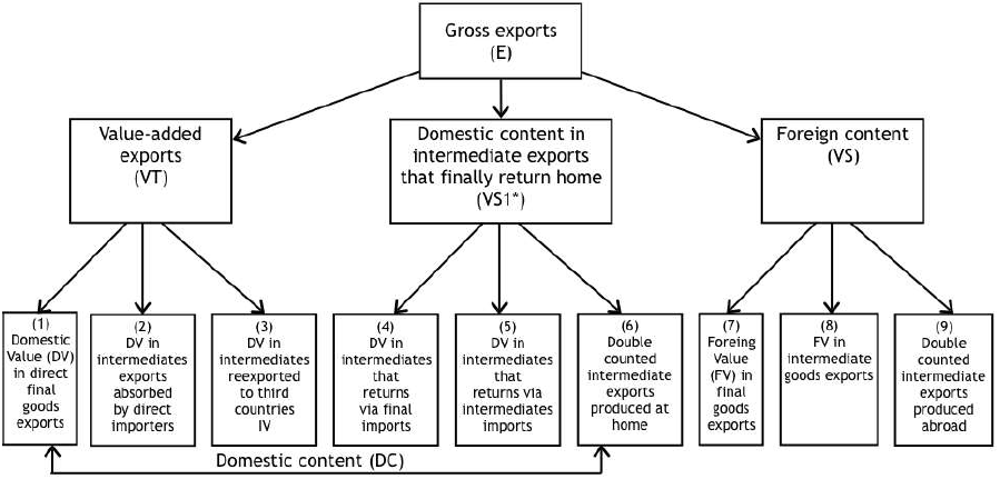
Source: Translation by the authors of the scheme of Koopman, Wang, & Wei (2014, p. 482).
Figure 1. Conceptual Framework of Koopman’s Export Decomposition
The previously defined block of exported value-added (VAX) can be subdivided into three types of goods:
Final goods. It is defined as the amount of national value-added in exports destined for consumption in the importing country. This is the case if there is a lack of productive co-production between countries.
Direct intermediate goods. It is defined as the amount of domestic value-added of exports of national goods made directly to the trading partner in order for the partner to continue the process of co-production of final goods destined to its domestic market.
Indirect intermediate goods. It is defined as the amount of domestic value-added of exports incorporated in intermediate goods that, instead of being processed and consumed as a final good in the immediate destination country, are re-exported to a third country. This productive process implies a productive chain that extends beyond the bilateral.
The previously defined block of returned domestic content that is exported and then re-imported (vS1*) can be subdivided into three subcategories:
Final goods. It is defined as the possibility of re-entry of nationally added value in exports in the form of final goods produced abroad.
Intermediate goods. Defined as the possibility that a part of the added value returns in the form of new intermediate goods, that is, the export of raw materials that undergo their initial transformation abroad and are then re-imported as intermediate industrial goods subject to new transformations.
Domestic double registration (DCI). Defined as the possibility that a fraction of the value-added returns to the country of origin in the form of intermediate goods. If these intermediate products are processed and exported again, their domestic value- added will have crossed the national border on more than one occasion.
The previously defined block of vertical integration (VS), or foreign content of exports, can be subdivided into three subcategories:
Final goods. Defined as the participation of imported final goods directly incorporated in exports.
Intermediate goods. Defined as the fraction of intermediate imported goods directly and indirectly re-exported.
Domestic double registration (DC2). Defined as the possibility that a fraction of the value-added is re-exported back to the country of origin in the form of intermediate goods in the case that the productive process allows goods to cross national borders several times, resulting in the double counting of the foreign content.
It is important to note that the methodology of Koopman, Wang, and Wei (2012; 2014) was designed for the breakdown of the value-added content in total aggregate exports in the multilateral case.
Stehrer (2013) proposes three modifications to the methodology of Koopman, Wang, and Wei (2014) to enable the components of value-added to add up precisely to the value of total bilateral exports. The three modifications in the multilateral and aggregate case are as follows:
Indirect value (IV). Defined as the amount of national added value contained in the exports that a country makes indirectly to its partner that does not form part of the gross bilateral exports from the first to the second (there will be an implicit bilateral trade flow without a commercial counterpart in the customs records). This proportion of bilateral VAX is called IV.
Final re-export value (RE-X). Defined as the amount of national value-added contained in the final exports that a country makes to its partner that is then re- exported to a third country. This trade flow does not have a counterpart VAX since this must be attributed to the third country. In other words, the trade flow to the partner must be accounted for, on the one hand, and the value-added flow (through indirect channels) to the third country, on the other.
Intermediate re-export value (RE-X1). Measures the amount of national value- added contained in the exports that a country makes to its partner that are then re- exported to a third country where they were not consumed but re-exported again. This new country will register value-added re-exports from the country of origin even if there are no bilateral gross exports nor VAX from the country of origin.
Thus, the RE-X—or proportion of value-added that passes through the trading partner and is later re-exported—may or may not have a bilateral trade flow as a counterpart. That is, only the fractions of bilateral VAX (IV) and RE-X will reach the trading partner through a bilateral export flow. Therefore, to ensure that the breakdown of total value-added adds up exactly to the bilateral gross exports, the transited value-added that the destination country received indirectly must be subtracted. However, this approach presents a disadvantage at the sectoral-bilateral level.
Wang, Wei, and Zhu (2013) propose another method for dividing value-added at the sectoral- bilateral level. This methodology modifies the disaggregation components of value-added that can be grouped in the three previous categories. In the section showing the breakdown of Wang, Wei, and Zhu (2013), we present the breakdown of this concept in 16 terms for the sectoral-bilateral case.
STATISTICAL SOURCES AND CONSTRUCTION OF THE BILATAERAL INPUT-OUTPUT TABLE
To conduct a sectoral-binational analysis of participation in the value chain using an input-output framework, we must ask the following: How should the input-output tables of the U.S. and Mexico be integrated and with the rest of the world? The answer is to develop a bilateral/inter-country input-output table between the U.S. and Mexico. In undertaking this task, it was considered appropriate that sectoral aggregation had the highest possible level of detail. For the U.S., the table constructed by IMPLAN (Minnesota Implan Group, 2017) for 2013 was used, with a sectoral structure of 526 sectors.
In the case of Mexico, we used the official national table for 2013 (INEGI, 2014) of the North American Industrial Classification System (Sistema de Clasificación Industrial de América del Norte [SCIAN]) composed of 261 sectors and disaggregated to the four-digit level. The official matrix was updated to 2013 to coincide temporally with the matrix for the U.S. and with the data for the year reflected in the 2014 Economic Census (INEGI, 2014).
The official update to the RAS methodology5 which, based on the base matrix and availability of the aggregate values by row and column for 2013, applied an iterative bi-proportional process with the aim of making the sum of the values of the sectoral interactions in the matrix coincide with the aggregates for the year to be estimated (Lahr & de Mesnard, 2004; INEGI, 2014). The aggregate data for the borders in 2013 were taken from the 2014 Economic Censuses (INEGI, 2014).
The first step to generate the integrated U.S.-Mexico model was to ensure the sectoral compatibility of the individual models. Of the 526 sectors, 488 corresponded fully at the four-digit level of the SCIAN, and the remaining 38 combined activities from several sectors. These were assigned a weight according to their relative participation in the aggregated data using data from the economic censuses. This process resulted in 259 sectors. Finally, to ensure the compatibility of activities between both models, minor adjustments of the classifications were required, resulting in 247 sectors of economic activity.
After both national models have a compatible classification, the second step was constructing the integrated model for the estimation of the trade flows between both countries at the level of individual sector interaction. However, for this, we have the aggregate flows of U.S.-Mexico trade as part of the matrix of import flows at the level of sector interaction and total aggregate exports by sector. A similar problem was faced when estimating the multiregional models in Canning and Wang (2005).
The reasoning behind the estimation of the foreign trade matrices begins by considering that trade between the two countries already forms part of the import and export aggregates of each country’s matrices. Therefore, their incorporation to the matrix initially requires subtracting the values of the trade flows from the total imports and exports in the matrices of both countries as appropriate.
With this procedure, we can incorporate these amounts to the trade matrices by making an initial distribution based on the structural composition of the import matrices for each country as appropriate. The consistency of the aggregates is achieved by considering that the sum of the rows of the trade flows between both countries and the exports should coincide with the exports by sector of the individual models; and, in turn, the sum of the columns of the trade flows between the U.S. and Mexico and the imports of the rest of the countries should add up by sector to the total imports of the individual matrices. Finally, the adjustment of the trade values and imports and exports of the rest of the countries can be achieved using the RAS method, which adjusts the sum of the previous values to the total aggregates by row and column.
The scheme of the bilateral input-output table is shown in Table 1. It is a combination of the sector interactions
(
| Millions of dollars | ||||||||
|---|---|---|---|---|---|---|---|---|
| Intermediate demand 1_/ | Final demand | |||||||
| s | r | s | r | ROW | ||||
| 1…J…247 | 1…J…247 | 1…k 4 | E | 1…k. 4 | E | Exp ROW | I=P | |
| 1 (I) | 1 (II) | (III) | (IV) | (XVII) | ||||
| s | i |
i |
0 | x s | ||||
| 247 | 247 | |||||||
| 1 (V) | 1 (VI) | (VII) | (VIII) | |||||
| r | i |
i |
0 | x r | ||||
| 247 | 247 | |||||||
| 1 (IX) | 1 (X) | (XI) | (XII) | |||||
| Imp ROW |
i |
i |
0 | 0 | 0 | 0 | ||
| 247 | 247 | |||||||
| 1 (XIII) | 1 (XIV) | (XV) | (XVI) | |||||
| VA | P |
P |
0 | 0 | 0 | 0 | 0 | GDP |
| 4 | 4 | |||||||
| I=P | x s | x r | ||||||
Source: Own elaboration.
1_/ abbreviations: s=country s; r=country r; ImpROW=imports from the rest of the world; VA=value added; Exp ROW=exports from the rest of the world; I=gross inputs; P=gross product; GDP=gross domestic product.
The balance sheet equations can be derived from Table 1 in matrix form as follows:
where xs is the total gross production in country
s destined as intermediate or final goods domestically or
internationally; xss is the intermediate demand in country
s for intermediate goods or inputs in country s;
yss is the final demand in country s for
final goods in country s; xrs is the
intermediate demand in country r for intermediate goods or inputs from
country s; y is the final demand in country
r for final goods from country s;
and
Based on Leontief’s assumption about the linearity of the parameters of the cost
function, i.e.,
Equations (2) and (4) represent the direct intra-country coefficients, and equations (3) and (5) are the inter-country trade coefficients. Substituting these structural equations into the balance equation and arranging them in the matrices, we obtain the following:
By rearranging the previous matrices, we obtain the following:
where bi,j are the Leontief inverse coefficients or total coefficients, ys = ysr + ysssup>, and yr = ysr + yrr. Thus, we obtain the solution for the Leontief system of equations for the intercountry case.
WANG, WEI, AND ZHU DECOMPOSITION
The division of sector-bilateral flows of the gross value-added of exports proposed by Wang, Wei, and Zhu (2013) is long and tedious. Because of the limited space, it is not possible to present the complete derivation. However, we show the breakdown of the 16 terms of gross export value- added and a simple interpretation of each component.
The breakdown of exports from country s to country r (ers) according to their value components by origin, destination, and final and intermediate goods, is as follows:
T1. |
Direct added value (DVA) of the exports of final products. |
T2. |
DVA of intermediate exports to importing country r that are finally consumed in that country. |
T3. |
DVA of intermediate exports to importing country r that are at the same time intermediate exports to third countries t for the production of final products with use in third countries. |
T4. |
DVA of intermediate exports to importing country r for final exports to third countries t. |
T5. |
DVA of intermediate exports to importing country r that are intermediate exports to third countries t. |
T6. |
DVA returned in final goods from importing country r. T7. DVA returned in final goods from third countries t. |
T8. |
DVA returned in intermediate imports. |
T9. |
Double counting of DVA to produce exports of final goods. |
T10. |
Double counting of DVA to produce exports of intermediate goods. |
T11. |
Value-added by the direct importer r in the final exports of country s. |
T12. |
Value-added by the direct importer r in the intermediate exports of country s. |
T13. |
Double counting of the value-added by direct importer r in the exports of country of origin s. |
T14. |
Value-added of third countries t in final exports. |
T15. |
Value-added of third countries t in intermediate exports. |
T16. |
Double counting of value-added from third countries (t, *) in exports from country of origin s. |
where vi is the value-added matrix of country i, bij is the sub-matrix of the inverse Leontief matrix, lij is the local Leontief inverse of the sub-matrix xij , T is transposed, and # refers to the multiplication of “element by element” similar to the point product of two vectors.
The terms can also be grouped as domestic value-added (DVA), foreign value-added (FVA), return value-added (RVA), and pure double counting (PDC).
DVA is equal to the sum of terms T1 to T5. This is the sum of the domestic value- added used in other countries.
RDV is equal to the sum of terms T6 to T8. It represents the exported value-added that eventually returns to the country of origin.
FVA is the sum of terms T11, T12, T14, and T15. It represents the portion of exports whose value-added comes from other countries (T11 and T12 for the direct importer; T14 and T15 for third countries).
PDC is the sum of terms T9, T10, T13, and T16. It represents double counting.
Total DVA is the sum of DVA and RDV. That is, the sum of all domestic value- added regardless of where it is eventually used.
EMPIRICAL ANALYSIS
The passage of NAFTA led to an increase in trade flows between member countries. It is currently a challenge to measure bilateral trade volumes because of the boom in global co-production chains at the bi-national level.
Given this context, we ask how the economic benefits of participating in bilateral co-production chains are distributed. Table 2 shows the results of the breakdown of the origin of the value-added of the gross exports of the U.S. and Mexico in 2013. For this, the “decompr” module developed by Quast and Kummritz (2015) integrated to the R software (R Core Team, 2018) was used.
Table 2. Results of the Breakdown of Value-Added Trade Between the U.S. and Mexico (In Millions of Dollars)
| Component | U.S (1) |
Mexico (2) |
|---|---|---|
| Domestic value-added in final exports | 46,358.1 | 61,712.4 |
| Domestic value-added in intermediate exports absorbed
by direct importers |
73,797.4 | 78,753.4 |
| Domestic value-added in intermediate exports
re-exported to third countries |
11,858.8 | 19,933.9 |
| Domestic value-added returning as final goods | 29,722.9 | 882.4 |
| Domestic value-added returning home as intermediate goods | 20,532.7 | 1,666 |
| Double counting of domestic origin | 6,426 | 1,470.9 |
| Foreign value-added in exports of final products from
the direct importer |
8,824 | 29,722.9 |
| Foreign value-added in exports of intermediate goods
from the direct importer |
1,666 | 20,532.7 |
| Double counting of foreign origin due to the export
production of the direct importer |
1,470.9 | 6,426 |
| Trade with the participating third countries | 43,309.5 | 65,852.5 |
| Total gross bilateral trade | 236,024.7 | 286,953 |
Source: Own elaboration based on the model of Wang, Wei, & Zhu (2013).
In 2013, of the U.S. $236 billion exported from the U.S. to Mexico, U.S. $120.2 billion corresponds with value-added directly in the U.S. and another U.S. $62.1 billion with value-added in the U.S. of inputs exported as intermediate goods that returned to the U.S. as exports. Additionally, U.S. $6.4 billion correspond with duplicate counting but are integrated to the national value-added of gross exports totaling U.S. $188.7 billion.
The other components of U.S. exports to Mexico are U.S. $2.5 billion of value-added in Mexico and U.S. $1.4 billion of duplicate accounting generated in Mexico. Finally, U.S. $43.3 billion of the value-added is imported by the United States from other nations to be integrated in exports to Mexico.
The results show that of the U.S. $287 billion in exports from Mexico to the U.S., the value- added directly in Mexico reaches U.S. $140.5 billion. To this, we must add U.S. $22.5 billion of value-added that returned to Mexico and U.S. $1.5 billion of double counting forming part of the U.S. $164.4 billion of domestic production contained in gross exports. The rest is made up of the U.S. $50.2 billion of value-added in the U.S. and a double counting in the U.S. of U.S. $6.4 billion. The U.S. $65.9 billion of imports from third countries must also be considered. These results are consistent with those of the Bank of Mexico (BANXICO, 2017).
In terms of domestic value-added, that of the gross exports from the U.S. reaches U.S. $188.7 billion dollars, while that of Mexico is around U.S. $164.4 billion. This has significant implications because it means that after discounting the imported amount from gross exports, the U.S. domestic content exceeds that of Mexico. Likewise, in terms of trade between both partners, the implication would be that the U.S. maintains a surplus in the trade balance with Mexico, as opposed to the conclusions derived from the traditional analysis of gross foreign trade between both countries.
In addition, there is a large difference between the domestic and foreign components of the value-added in exports. For the U.S., the foreign value-added in its exports reaches U.S. $2.5 billion dollars, whereas for Mexico, this amount reaches U.S. $50.2 billion, more than 20 times the amount for the U.S.
It can also be observed that the amount of imports from other countries is greater for Mexico, reaching U.S. $65.9 billion dollars, in comparison to U.S. $43.3 billion for the U.S. This means that a significant proportion of the gross bilateral trade surplus (U.S. $22.5 billion, or 44%) comes from other countries in the form of intermediate imports. In other words, the gross bilateral surplus does not take into account that, through GVCs, Mexico imports U.S. $22.5 billion in excess of what the U.S. imports for the production of exported goods and, consequently, the trade surplus increases considerably.
On the other hand, the analysis of these figures in aggregate per concept and in relative terms can be carried out by calculating the indexes used by the abovementioned authors (Koopman, Wang, & Wei, 2012) who previously researched the extent of value-added content in exports. The results are presented in Table 3.
Table 3. Breakdown of Value-added and Relative Indicators of Trade Between the U.S. and Mexico (Millions of Dollars)
| Breakdown of value-added | U.S. to Mexico | Mexico to U.S. |
|---|---|---|
| Value-added in exports | 120,155.5 | 140,465.8 |
| National added value | 161,737.2 | 161,282.0 |
| Foreign added value | 2,548.4 | 50,255.6 |
| National content in gross exports | 188,695.9 | 164,418.9 |
| Double counting of pure national origin | 6,426.0 | 1,470.9 |
| Double counting of pure foreign origin | 1,470.9 | 6,426.0 |
| Trade with participating third countries | 43,309.5 | 65,852.5 |
| Relative indicators | ||
| Relationship of added value to export
value (Johnson & Noguera, 2012a) |
0.5091 | 0.4895 |
| Value-added in exports | 0.6853 | 0.5621 |
| Value-added in exports | 0.7995 | 0.5730 |
| Total gross bilateral trade | 236,024.7 | 286,953.0 |
Source: Own elaboration based on the model of Wang, Wei, & Zhu (2013).
The table shows that, in both domestic value-added content and total domestic content, the trade relationship favors the U.S. and indicates a surplus for the country given that the value of its exports exceeds that of its imports. There are also notable differences in the foreign value-added content of each country’s exports. For the U.S., it only reaches U.S. $4 billion of the content of imports in its exports. For Mexico, the import content from the U.S. in its exports reaches U.S. $56.7 billion, which is only 30% of the domestic content of exports to the U.S.
In terms of the proportion of value-added proposed by Johnson and Noguera (2012b) (VAX ratio) applied to U.S.-Mexico trade figures, the value reaches 51% for the U.S. and 50% for Mexico. In regard to the proportions of domestic value-added and domestic content in gross exports, these reach nearly 80% in the U.S. and 57.3% in Mexico.
The results of the relative indices show how the consideration of trade volumes in terms of value-added only partially accounts for a country’s participation in international trade. Also, after integrating the returned value-added, a country’s trade position can change, as occurs in the U.S.-Mexico trade relationship. In addition, it is important to recognize how imports from other countries are an important figure that can explain part of the trade in gross terms between countries. The integration of these figures enables a closer examination of the contributions of each country and third parties in international trade relations.
The findings per sector are shown in Table 4. The information in the table shows how trade between the two countries is highly concentrated, with exports in the top 15 sectors accounting for more than 58% of exports of the total 247 sectors. In terms of value-added, for most sectors, the percentage is lower than average, although these produce inputs to a wide variety of processes.
Table 4. Results of the Breakdown of Value-Added in U.S. and Mexican Trade by Major Sector (Millions of Dollars)
| Domestic content | Foreign content | Gross bilateral trade |
||||||||||
|---|---|---|---|---|---|---|---|---|---|---|---|---|
| Domestic value-added (DVA) | Double counting |
Foreign value-added (FVA) | Double counting |
|||||||||
| NAICS | Description | Value-added in exports | DVA reexportad |
DVA re- exported |
Rest of the world |
|||||||
| DVA_FIN | DVA_INT | DVA_INTrex | RDV_FIN | RDV_INT | DDC | MVA_FIN | MVA_INT | MDC | ||||
| 3344 | Manufacture of electronic components | 678 | 2 841 | 2,136 | 5 518 | 2 949 | 818 | 13 | 55 | 227 | 2 983 | 18 220 |
| 3241 | Manufacture of oil and coal products | 0 | 8,784 | 701 | 543 | 725 | 191 | 0 | 600 | 149 | 6 381 | 18 073 |
| 3363 | Manufacture of parts for motor vehicles | 286 | 5,996 | 971 | 4,630 | 1,226 | 370 | 6 | 128 | 155 | 3 065 | 16 832 |
| 3251 | Manufacture of basic chemical products | 316 | 6,283 | 564 | 691 | 1,326 | 328 | 7 | 131 | 61 | 2 377 | 12 083 |
| 3252 | Manufacture of synthetic resins and rubber, and chemical fibers |
0 | 3,152 | 524 | 1,229 | 1,366 | 313 | 0 | 64 | 71 | 1 856 | 8 574 |
| 3361 | Manufacture of cars and trucks | 5,660 | 39 | 8 | 50 | 7 | 2 | 251 | 2 | 3 | 1 914 | 7 937 |
| 3342 | Manufacture of communication equipment | 2,551 | 530 | 432 | 1,294 | 587 | 180 | 51 | 11 | 51 | 1 978 | 7 665 |
| 3341 | Manufacture of computers and
peripheral equipment |
2,302 | 1,511 | 441 | 995 | 561 | 154 | 48 | 31 | 45 | 1 466 | 7 554 |
| 3339 | Manufacture of other machinery and equipment for general industry |
3,162 | 1,323 | 182 | 303 | 410 | 112 | 62 | 26 | 20 | 1 169 | 6 771 |
| 3345 | Manufacture of measurement, control, navigation, and medical electronic equipment |
2,227 | 889 | 336 | 891 | 609 | 176 | 33 | 13 | 30 | 1 006 | 6 208 |
| 3336 | Manufacture of internal combustion engines, turbines, and transmissions |
263 | 2,129 | 413 | 957 | 640 | 249 | 8 | 62 | 67 | 1 267 | 6 055 |
| 3261 | Manufacture of plastic products | 605 | 2,008 | 347 | 868 | 621 | 158 | 9 | 28 | 28 | 914 | 5 587 |
| 3353 | Manufacture of power generation and distribution equipment |
676 | 1,219 | 379 | 815 | 961 | 274 | 19 | 34 | 68 | 994 | 5 441 |
| 3329 | Manufacture of other metal products | 150 | 1,867 | 334 | 848 | 932 | 263 | 2 | 29 | 37 | 779 | 5 240 |
| 3359 | Manufacture of other
electrical equipment and accessories |
470 | 1,144 | 376 | 981 | 816 | 235 | 14 | 34 | 73 | 1 040 | 5 183 |
Source: Own elaboration based on the model of Koopman, Wang, & Wei (2012).
In that sense, as stated above, the largest difference rests in the exports returned to the U.S. economy as intermediate products that are then integrated into U.S. products and exported again. This is the case, for example, of electronics components manufacturing (sector 3344), which accounts for 46.5% of the U.S. $18 billion of gross exports. However, of this amount, U.S. $5.7 billion is domestic value-added, U.S. $8.5 billion is returned value-added, and U.S. $3 billion is imports from third countries. These latter amounts explain U.S. $17 of the U.S. $18 billion dollars traded.
We must also consider sectors such as motor vehicle parts manufacturing (sector 3363), which have low added value but have strong sectoral links with other sectors of the Mexican economy. This sector can generate U.S. $7.3 billion dollars of domestic value-added of the U.S. $16.8 billion dollars exported, of which an additional U.S. $5.9 billion dollars are returned value-added. That is, of the U.S. $16.8 billion exported, although less than 50% is domestic, more than 75% is value- added in the U.S. during the GVC process.
The correct measurement of the value-added in exports between these two countries is a basic starting point for assessing the effects of any changes to trade policy. How would the renegotiation or cancellation of NAFTA affect participation in bilateral co-production chains? The answer can be found in the following graph in which the circles on the line indicate sectors for which the proportion of value-added is equal between countries. In this case, there is no domestic value returning in intermediate imports. The majority of the sectors in the case of Mexican exports are located near this line. In contrast, in the case of U.S. exports, a large part of the sectors are located above the line, especially the sectors with lower domestic value on the horizontal axis, thus increasing the domestic content considerably.

Source: Own elaboration based on the results.
Graph 1. Total Domestic Value-Added of Mexican and U.S. Exports.
This result is relevant because it means that during NAFTA an important part of the income from Mexican exports was destined to remunerate productive factors employed in the U.S. As a consequence, the multiplier effect—direct and indirect—associated with any change in binational exports is greater for the U.S. than Mexico.
CONCLUSIONS
In the present analysis, we highlight that, although Mexico has officially had a surplus trade balance with the U.S. during the NAFTA period, there is evidence of a deficit in terms of the value- added in gross exports. The figures describing the flow of added value gross exports from Mexico to the U.S. reach 164.4 billion dollars, while the domestic content of gross exports from the U.S. is $188.7 billion.
The main difference is between the domestic and foreign components of the value-added in exports. For the U.S., the foreign value-added in its exports reaches $2.5 billion, while for Mexico it is around $50.2 billion, or 20 times higher than the amount of the U.S. One conclusion directly derived from this finding is that, as a consequence of NAFTA, a significant part of the income from Mexican exports goes to remunerate production factors employed in the United States.
Bilateral trade is highly concentrated in 15 export sectors that account for more than 58% of exports. In particular, the electronics manufacturing sector stands out, representing 46.5% of trade, of which U.S. $18 billion dollars correspond with gross exports, U.S. $5.7 billion with domestic value-added, $8.5 billion with returned value-added, and $3 billion with imports from third countries, explaining $17 of the $18 billion dollars traded.
In addition, the vehicle parts manufacturing sector (sector 3363) also has a high domestic content of gross exports. Of the U.S. $16.8 billion exported, $7.3 billion are domestic value-added and 5.9 billion are returned value-added. Based on these findings, the importance of the difference in the consumption of intermediate goods between both countries can be highlighted in addition to the consequences for the added value generated in certain sectors of activity.
Therefore, the correct measurement of the value-added in bilateral sectoral exports should be a basic starting point for assessing the appropriateness or effects of any changes to binational trade policy. On the Mexican side, where a greater amount of foreign content is generally observed in production (and exports), the electronics, oil refining, chemical and plastic production, base metals, and metal-mechanics sectors stand out with a proportion of approximately 40%. The contribution of the U.S. side, which is usually the main source of this foreign content, has generally been on the rise.
For the U.S., the proportion of foreign content in all cases is around 20%, whereas that explained by Mexico never exceeds 3% (the highest being in the automotive sector). This is partly explained by the asymmetric economic relationship. As a result, the multiplier effect—direct and indirect—associated with any change in binational exports is greater for the U.S. than for Mexico.
Finally, an important limitation to be taken into account in future studies that aim to estimate the value-added in the trade relations between the two countries is the need to incorporate the impact of the rest of the world endogenously in the net balance of the distribution of value-added at the disaggregated level presented herein. In the case of the countries considered herein, the importance of this aspect is truly evident and, ultimately, it cannot be said that third countries are taking advantage of trade agreements without taking into account their impact. However, without a doubt, the estimation is complex.
REFERENCES
Amar, A. y García Díaz, F. (2018). Integración productiva entre Argentina y el Brasil: Un análisis basado en metodologías de insumo-producto interpaís. Santiago, Chile: Naciones Unidas/Comisión Económica Para América Latina. Recuperado de https://www.cepal.org/es/publicaciones/43623-integracion-productiva-la-argentina-brasil-un-analisis-basado-metodologias [ Links ]
Baldwin, R. y Lopez‐Gonzalez, J. (2015). Supply‐chain trade: A portrait of global patterns and several testable hypotheses. The World Economy, 38(11), 1682-1721. [ Links ]
Banco Nacional de México (Banxico). (2017). Análisis del Balance Comercial Manufacturero de Estados Unidos con México en Términos de Valor Agregado. Extracto del Informe Trimestral Julio-Septiembre. [ Links ]
Canning, P. y Wang, Z. (2005). A Flexible Mathematical Programming Model to Estimate Interregional Input-Output Accounts. Journal of Regional Science, 45(3), 539-563. [ Links ]
Daudin, G., Rifflart C. y Schweisguth, D. (2011). Who produces for whom in the world economy? Canadian Journal of Economics/Revue canadienne d'économique, 44(4),1403- 1437. [ Links ]
De Mesnard, L. (1989). Note about the theoretical foundations of biproportional methods. En Ninth International Conference on Input-Output Techniques, 4 y 5 de septiembre, Keszthely, Hungría. [ Links ]
Hummels, D., Ishii J. y Yi, K. M. (2001). The nature and growth of vertical specialization in world trade. Journal of international Economics, 54(1 ), 75-96. [ Links ]
Instituto Nacional de Estadística y Geografía (Inegi). (2014). Sistema de Cuentas Nacionales de México. Desarrollo de la matriz de insumo producto 2012: Fuentes y Metodología. Recuperado de http://www.inegi.org.mx/est/contenidos/proyectos/cn/mip12/doc/SCNM_Metodologia_28.pdf [ Links ]
Johnson, R. C. (2014). Five facts about value-added exports and implications for macroeconomics and trade research. Journal of Economic Perspectives, 28(2), 119-42. [ Links ]
Johnson, R. C. y Noguera, G. (2012a). Accounting for intermediates: Production sharing and trade in value added. Journal of international Economics, 86(2), 224-236. [ Links ]
Johnson, R. C. y Noguera, G. (2012b). Proximity and production fragmentation. American Economic Review, 201(3), 407-11. [ Links ]
Koopman, R., Wang, Z. y Wei, S. J. (2008). How Much of Chinese Exports is Really Made In China? Assessing Domestic Value-Added When Processing Trade is Pervasive. National Bureau of Economic Research Working Paper Series , (14109). Recuperado de https://www.nber.org/papers/w14109.pdf [ Links ]
Koopman, R., Wang, Z. y Wei, S. J. (2012). Tracing Value-Added and Doubled Counting in Gross Exports. National Bureau of Economic Research Working Paper Series, no. 18579. Recuperado de https://www0.gsb.columbia.edu/mygsb/faculty/research/pubfiles/5852/w18579.pdf [ Links ]
Koopman, R., Wang, Z. y Wei, S. J. (2014). Tracing value-added and double counting in gross exports. American Economic Review, 104(2), 459-94. Recuperado de https://www.aeaweb.org/articles?id=10.1257/aer.104.2.459 [ Links ]
Lahr, M. L. y de Mesnard, L. (2004). Biproportional Techniques in Input-Output Analysis: Table Updating and Structural Analysis. Economic Systems Research, 16 (2), 115- 134. doi: 10.1080/0953531042000219259 [ Links ]
Minnesota Implan Group (MIG). (2017). United States 2013 lmplan data. Minnesota: Stillwater. [ Links ]
Quast, B.A. y Kummritz, V. (2015). Decompr: Global Value Chain decomposition in R. CTEI Working Papers, 1 . [ Links ]
R Core Team. (2018). R: A language and environment for statistical computing. R Foundation for Statistical Computing. Viena. Disponible en http://www.R-project.org/ [ Links ]
Solaz, M. (2016). Cadenas globales de valor y generación de valor añadido: el caso de la economía española. Working Papers. Serie EC 2016-01, Instituto Valenciano de Investigaciones Económicas, S.A. (Ivie) . Recuperado de https://web2011.ivie.es/downloads/docs/wpasec/wpasec-2016-01.pdf [ Links ]
Stehrer, R. (2013). Accounting relations in bilateral value added trade. Working papers, 101, Wiener Institut für Internationale Wirtschaftsvergleiche , Viena. Recuperado de https://wiiw.ac.at/accounting-relations-in-bilateral-value-added-trade-dlp-3021.pdf [ Links ]
Timmer, M. P., Los, B., Stehrer, R. y De Vries, G. J. (2013). Fragmentation, incomes and jobs: an analysis of European competitiveness. Economic policy, 28(76), 613-661. [ Links ]
Trefler, D. y Zhu, S. C. (2010). The structure of factor content predictions. Journal of International Economics, 82(2), 195-207. [ Links ]
Wang, Z., Wei, S. J. y Zhu, K. (2013). Quantifying International Production Sharing at the Bilateral and Sector Levels, NBER Working Papers 19677. National Bureau of Economic Research Inc. Recuperado de http://www.nber.org/papers/w19677.pdf [ Links ]
West, J. (2018). Asian Century… on a Knife-edge. Singapore: Palgrave Macmillan. [ Links ]
Xing, Y. y Detert, N. (2010). How the iPhone Widens the United States Trade Deficit with the People’s Republic of China. Asian Development Bank Institute Working Paper Series. No. 257 . Tokyo: Asian Development Bank Institute. Recuperado de http://www.adbi.org/working-paper/2010/12/14/4236.iphone.widens.us.trade.deficit.prc/ [ Links ]
4Other studies take gross export flows assuming a given use (intermediate or final) from available foreign trade statistics (Harmonized System, Uniform International Trade Classification, or tariff nomenclators). Meanwhile, the input-output table shows the interrelationships between sectors and allows for tracing the origin of the flows of gross production necessary to generate a unit of final demand. From these production flows, the value-added generated by sector/country can be obtained by multiplying the production necessary to satisfy certain levels of final demand by the corresponding proportion of value-added over gross production (Amar & García Díaz, 2018).
5This is a translation of the matrix adjustment theory with restrictions on the estimation of input- output matrices (row and column totals). The adjustment was first used as a technique to update the matrix of intermediate transactions (de Mesnard, 1989).
Received: April 02, 2019; Accepted: September 18, 2019
 Este es un artículo publicado en acceso abierto bajo una licencia Creative
Commons
Este es un artículo publicado en acceso abierto bajo una licencia Creative
Commons
