Artículos

 

Tijuana's Dynamic Unemployment and Output Growth

 

Alejandro Díaz-Bautista*

 

*Professor of economics, researcher and economic consultant, El Colegio de la Frontera Norte. Dirección electrónica: gus12052000@yahoo.com.

 

Artículo recibido el 5 de marzo de 2002.
Artículo aceptado el 20 de noviembre de 2002.

 

Abstract

During the 1990s, Mexico successfully implemented a program of economic reforms and free trade aimed at a complete restructuring of its economy. Surprisingly, the reform process seems to have had little impact on unemployment. An analysis of trends indicates that, even in the worst years of economic crisis, average unemployment rates in Mexico did not exceed 7.4% (reached in the third quarter of 1995). Tijuana's unemployment rate averaged 0.725% in 2001, when the economy was experiencing the start of a recession and major structural reforms were expected. These figures seem very low when compared to those for other countries. This article's goal is to evaluate transitory demand shocks and permanent supply shocks in Tijuana's unemployment time series, as given by that identification restriction and the structural break unit root methodology. Okun's Law is also tested for the Tijuana unemployment series.

Keywords: 1. unit root, 2. output, 3. unemployment, 4. Tijuana, 5. Mexico.

 

Resumen

En la década pasada, México estableció un programa de reformas económicas y de libre comercio encaminadas a la completa reestructuración de su economía. sorprendentemente, el proceso de reforma tiene poco impacto en el desempleo. Un análisis de las tendencias indica que, aun en los peores trimestres de la crisis económica, la tasa de desempleo promedio no fue mayor de 7.4%. La tasa de desempleo trimestral de la ciudad de Tijuana en 2001 alcanzó en promedio 0.725%, en un período donde inició una recesión en la economía. Estas cifras son bajas al ser comparadas con las de otros países. El objetivo del estudio es evaluar los choques transitorios de la demanda y los permanentes de la oferta en el desempleo en Tijuana en diferentes períodos. Para ello utiliza la restricción de identificación y la metodología de raíz unitaria con corte estructural. La ley de Okun también es verificada para conocer la evolución del desempleo en Tijuana.

Palabras clave: 1. raíz unitaria, 2. producción, 3. desempleo, 4. Tijuana, 5. México.

 

INTRODUCCTION

Econometric time series analysis of unemployment in Mexico is quite rare. This article provides empirical evidence about the dynamics of Tijuana's labor market, which researchers consider one of the most important social laboratories in the world for the analysis of unemployment. The structural changes in the Mexican economy during the past 15 years had surprisingly little effect on the country's unemployment, which has been low even in the worst years of the adjustment process. The most striking feature of the structural reform is Mexico's range of employment growth rates across its primary and border cities and the similarity of trends in urban unemployment.

Employment shocks may have permanent effects in Tijuana. A city like Tijuana that experiences a demand shock that causes acceleration or slowdown in growth can expect to return to the same economic growth rate but on a permanently different path and level of unemployment. Unemployment patterns in Mexico's largest cities move from above to below the national average and vice versa.

From a welfare perspective, it matters greatly whether the cost of unemployment is widely spread or whether it falls primarily on a few. Even if only a small fraction of the labor force is unemployed at any point, these individuals may have specific characteristics that would make them particularly and repeatedly vulnerable. Another issue revolves around the relative importance of long-term unemployment and how demand and supply shocks affect unemployment. Specifically, one would want to know whether most unemployment is associated with normal turnover (movements from one job to the next) or if it is comprised primarily of individuals who are out of work for long periods.

A number of general results show that the dynamic effects of supply and demand in Tijuana are different from those Blanchard and Quah (1989) found for the United States. In particular, Tijuana's economy seems to show nominal and real rigidities, with no clearly shaped patterns in the responses to demand and supply disturbances of the analyzed variables, primarily unemployment. Among the recognized recessions and expansions in Mexico after 1987, the 1994 downturn was the one most identified as a supply driven shock (that is, it had a permanent effect on output, whereas demand shocks had a permanent effect on unemployment). The article's next section offers a brief discussion of Mexico's unemployment, and the subsequent section discusses the Tijuana region, unemployment data, and estimation procedures and results.

 

MEXICO'S UNEMPLOYMENT

Starting in the late 1980s, Mexico's economic liberalization produced long-term structural changes in the economy, which generated unemployment. Then, in 1995, nearly a million jobs were lost in the wake of the 1994 peso crisis. In August 1995, however, the economy began to replace those lost jobs. After eight years of massive downsizing and restructuring, the manufacturing sector started to create jobs in spring 1997. From a peak of 7.4% in the third quarter of 1995, unemployment, as measured by the official open unemployment rate, fell to 4.29% in the first quarter of 1997. However, the open unemployment rate, the official figure cited by the government, understates true unemployment in Mexico. As defined by the International Labor Organization, the open unemployment rate counts individuals who actively sought employment or attempted to perform a work activity on their own and who did not work even one hour per week during the survey period. Thus, the numbers do not reflect discouraged and underemployed workers, a group estimated to represent more than one-fifth of Mexico's economically active population. This may be why Tijuana's unemployment rate in 2001 averaged 0.725%, a low number considering that the economy was experiencing the start of a recession.

 

DATA ANALYSIS, EMPIRICAL EXERCISES, AND RESULTS

Despite the rapid and far-reaching reforms in Mexico during the trade liberalization and economic reform era, which have had a clear impact on the labor market, unemployment has remained fairly low throughout the adjustment process. Official statistics, drawn from the government census and from employment surveys, report a low unemployment rate for Mexico as a country (as low as 2.9% in the third quarter of 1991). An analysis of the trends indicates that during the 1990s, unemployment rates in Tijuana did not exceed 2.8%. These figures, surprisingly low by international standards, raise a number of questions about the nature and importance of unemployment in Mexico's primary cities, like Tijuana.

From January 1991 to January 1996, Tijuana's private sector saw the creation of 63,100 jobs. This is indicative of trends in the region. Tijuana's job creation comes mainly from the manufacturing sector. The growth of the manufacturing assembly plant (maquiladora) industry in the Tijuana-Rosarito corridor has played an important role in the local economy. Since its appearance in the region 34 years ago, the maquiladora sector has grown impressively, and it accounted for 48% of all job creation from 1980-1990. During 1990, the Tijuana-based maquiladoras accounted for as much as US$500 million in foreign exchange earnings.

Because of the significant presence of manufacturing, in particular, the maquiladora sector, and the proximity to the United States, Baja California represents a market different from other states in Mexico. Its economy is relatively isolated from the national economy and has developed largely through its connections to the U.S. economy. Output growth is thought to be higher and unemployment to be lower than elsewhere. Consequently, when the economic crises struck Mexico in the 1980s and early 1990s, and real wages fell by as much as 50%, Mexican labor rates became competitive on a global scale, leading to considerable growth in the number and size of maquiladoras in Baja California. The crisis of late 1994 and the implementation of the North American Free Trade Agreement (NAFTA) also had a positive effect on the number of maquiladoras in the state. New investment in Tijuana's maquiladora industry increased as Asian companies, especially from Japan and Korea, began to establish plants to produce inputs. From 1991 to 1999, the number of assembly plants in Baja California increased by 404, or more than 50% (see Table 1).

By 1998, maquiladoras accounted for 34% of the national total in terms of industrial factories and 21% in terms of jobs. Value added in Baja California accounted for 22% of the nation's total value added, or almost US$10 billion that entered the country as a result of maquiladora activity. In the fourth quarter of 2000, the city of Tijuana accounted for more than 64% of the Baja California assembly plants, and 68% of the state workers (see Table 2 and 3). However, in 2002, the U.S. economic deceleration caused the Baja California plants to operate at only 70% of capacity, significantly affecting the region's output growth. Because of the U.S. economic recession, the effects of nafta art. 303,¹ and generally excessive regulation, 60 000 workers lost their jobs.

Even with the loss of workers in the assembly plant maquiladoras, the unemployment rate remained at low levels. Mexico's national rate of open unemployment in the first quarter of 2002 was approximately 2.8%, whereas the rate for Tijuana in the same quarter was approximately 2.1%. The Instituto Nacional de Estadística, Geografía e Informática (INEGI, a government agency) emphasized that Tijuana has one of the lowest unemployment rates in Mexico, and it has sustained its economic growth despite of the recent world economic recession. The average quarterly unemployment rate in Tijuana between 1987 and 2002 was 1.19% whereas in Mexico City, it was almost double that, close to 2.1%.

During August 1999, Tijuana's unemployment rate was only 0.5%, while San Diego's was 3.3%, according to the U.S. Bureau of Labor Statistics Local Area Unemployment Statistics. Despite San Diego having its lowest unemployment rate since the 1950s, that rate was still six times higher than the rate in Tijuana in 1999.

One explanation for the difference in measured unemployment rates is the large informal economy and the absence of unemployment insurance benefits in Tijuana (rather than differences in concept or methodologies for making measurements). With some relatively minor variations, both the United States and Mexico follow accepted international practices for measuring unemployment. Both countries primarily rely on household surveys. In Mexico, the survey is conducted in the 40 largest metropolitan areas. In the United States, the survey is conducted nationally and includes places of all sizes. Mexico's omission of smaller urban areas and rural areas causes the measured rate to be higher than it would be otherwise, since those areas tend to have lower unemployment rates.

Unemployment is defined as the percent of the labor force that is currently without employment. National definitions vary, however, because definitions of the labor force and employment vary. In the United States, according to the U.S. Department of Labor, Bureau of Labor Statistics (2001) the labor force is considered to be the non-institutionalized population, 16 years or older, that is either working or actively looking for work. Individuals are classified as unemployed if they do not have a job, have actively looked for work in the prior four weeks, and are currently available for work. Mexico's definition considers the population that is 12 years or older, because it is recognized that young teenagers are often valuable contributors to family income. Neither country counts the population that has stopped looking for work (the so-called discouraged workers) as part of the labor force. Both countries also define "employment" as one hour of work for pay during the referenced week.

Another minor difference between Mexico and the United States concerns laid-off workers who are waiting to return to work or who expect to start a job within a month. In Mexico, these workers are categorized as employed whereas in the United States, they are categorized as unemployed.

Two key facts stand out about Mexico's labor market: First, half the country's population is younger than 21 years of age, with one third younger than 14, and one million people enter the work force each year. Second, the average Mexican has fewer than eight years of formal schooling, meaning that strong competition exists among workers for low-skilled jobs and among companies for highly skilled individuals. Mexico has based much of its development strategy on successfully attracting low-skill, low-wage manufacturing jobs from the United States and other countries. Mexico's labor market is estimated at 40 million out of a population of 99 million people, that is, approximately 42% of the Mexican population is economically active, compared to 47% in the United States. But the relative scarcity of low-skilled jobs means that, compared to the United States, there is a large pool of labor willing to be employed at significantly lower wage levels and under less stringent labor laws.

This labor pool and Mexico's youthful demographic profile are among Mexico's chief competitive advantages, particularly given Tijuana's proximity to the United States. Much of the foreign direct investment that has entered Mexico in recent years has come from companies hoping to reduce labor costs while manufacturing goods for export to the United States. The best example is the maquiladora assembly-for-export industry, but this is true for other industries as well. Tijuana and Ciudad Juárez, both border cities, are leading maquiladora centers that have extremely low unemployment rates compared to the rest of North America.

 

DATA AND VAR METHODOLOGY

This article uses unit roots and var econometric methodologies to analyze quarterly data for Mexican unemployment (u) and output growth (Dy). The data comes from the Encuesta Nacional de Empleo Urbano (Urban Labor Force Survey, ENEU), a household-based survey of 16 urban areas, and data from the Encuesta Nacional de Empleo, ENE (National Employment Survey). The sample used in the article is a quarterly time series, from the first quarter of 1987 through the fourth quarter of 2001. Unemployment is measured in percentage terms, whereas output growth is given by the quarterly real output level (Y), as INEGI reported it. Both series are from the INEGI website. The ENEU's main drawback is its limited coverage, providing no information on the population from rural areas or smaller urban centers. The ENE sample covers other main urban areas and a sample of the rural population but is performed only every 2 to 3 years. The econometric data analysis uses a quarterly unemployment time series obtained from INEGI, since this is the only one that covers the period analyzed. The article does not use the alternative measures of unemployment because of the limited number of observations and the unavailability of data.

The unemployment rate in Mexico has consistently been higher among women than among men. In 1983, the unemployment rate for men reached 5.3%, while that for women stood a full 2% points higher, at 7.6%. The numbers show that unemployment rates in Mexico are highest for the young, particularly for those 16 to 25 years of age. In 1988, the unemployment rate for males aged 16 to 20 stood at 8.4%, while for males 21 to 25, it was 5.3%, compared to an average male unemployment rate of 3.4%. Similarly, for women aged 16 to 20, the unemployment rate in 1988 was 14%, and for those aged 21 to 25, 8.9%, while the female average was 6.3%. By educational attainment categories, the highest unemployment rates for males correspond to those with either incomplete or complete low secondary schooling (7-9 years of schooling). For women, the highest rates correspond to those who have completed either low secondary (9 years) or higher secondary (10-12 years) levels of education.

Unemployment figures are based upon a strict definition of unemployment: An individual is unemployed only if he or she is actively searching for a job. However, research on other countries suggests that the distinction between "unemployed" and "not in the labor force" (based on intensity of search) is often very weak.

A positive feature of the ENEU is its use of a quarterly rotation system, with each rotation group (of households) remaining in the survey for five consecutive quarters. In Mexico, 25% of all unemployment spells for men and 53% for women end in the individual's withdrawal from the labor force. As is the case in the United States, these fractions are higher for those under 20 years of age: 37% of periods of unemployment for males aged 16 to 20 end in withdrawal from the labor force, while the comparable figure for women is 55%. A large fraction of those who withdraw (55% of males and 41% of females) reenter the labor force within three months. This suggests that at any point the distinction between "unemployed" and "out of the labor force" is difficult to observe for certain groups.

This implies that the official definition of unemployment in Mexico, which includes only those individuals who report that they are actively searching for a job, will tend to underestimate the true number of people who are, in fact, jobless.² The analysis of the individual survey responses from the ENEU reveal a large fraction of men who report being idle: These individuals are out of work, able to work, not studying, and not taking care of the household. The choice of definition can have important implications for the analysis of the structure and characteristics of unemployment.

Given Mexico's low official unemployment figures, even during adjustment, we must ask whether the official definition of unemployment adequately describes the depth and breath of the phenomenon. In other words, is unemployment properly measured? From a welfare perspective, it matters greatly whether the cost of unemployment is widely spread or whether it falls primarily on a few. Even if only a small fraction of the labor force is unemployed at any point in time, these individuals may have specific characteristics that would make them particularly and repeatedly vulnerable, and therefore, deserving of special attention.

The official INEGI definition of unemployment leads to underestimating joblessness, because it ignores short spells out of the labor force and transitions in and out of the labor force, which are common. The duration of unemployment is longer for older workers but does not vary substantially according to educational attainment. Heads of households and individuals with household responsibilities tend to exit from unemployment faster. Although the typical spell of unemployment is relatively short, almost 70% of all unemployment in the 1990s was attributable to spells lasting at least six months, and 30% corresponded to spells lasting at least a year. Although unemployment rates in Mexico, as measured over a one-week period, are low (3 to 6%), 15 to 20% all the members of the labor force experience at least one spell of unemployment over a year.

Mexico's overall age structure of unemployment is broadly similar to that observed for other countries. Unemployment rates are highest for the young, particularly for those 16 to 25 years of age, and they have been consistently higher among women than among men. However, the pattern of higher unemployment rates for secondary school graduates differs somewhat from that observed in other developing and industrialized countries, where unemployment appears to be more prevalent among the less educated.

Using the standard definition of unemployment (corresponding to the official rate in Mexico), men under age 25 account for as much as 60% of total unemployment. The comparable fraction for women is even higher, about 77%. As regards education, 53% of total male unemployment and 62% of total female unemployment corresponds to individuals with some form of secondary education. Individuals who have completed their secondary education account for 20% of total male unemployment and about 19.7% of total female unemployment. This suggests that the reservation wage and, possibly, family income are important determinants of unemployment in Mexico: More educated individuals will tend to have both a higher reservation wage and more family income, which would allow them to afford longer job-search periods. Future research could be done using the reservation wage as an important determinant of unemployment in Mexico. For this article, however, the analysis centers on the dynamics of unemployment.

To estimate the Vector Autoregression (var) of unemployment and output, both series have to be stationary. Assuming that to be the case, the reduced-form system can be rewritten in its moving-average representation, linking the current values of the series to contemporaneous and past reduced-form residuals. Given that, we must choose the appropriate lag length. Blanchard and Quah (1989) is the seminal work and a classic in the literature of structural vars. Their contribution refers to the restriction used to identify permanent and transitory innovations, often called supply and demand disturbances, where the latter is assumed to have no long-run effects in the output level, contrary to the former. Several studies have applied the same kind of identification. For example, Enders and Lee (1997) decompose real and nominal shocks to the exchange rates; Gamber (1996) estimates aggregate demand and supply curves; and Gamber and Joutz (1993) replicates the original work with an industrial product index instead of gdp. Additionally, Blanchard and Katz (1992) examine the general features of regional booms and slumps, studying the behavior of unemployment for states in the United States. They try to answer how the typical U.S. state has been affected by an adverse shock to employment, and how it has adjusted. This section tries to analyze the general features and behavior of Mexico and Tijuana's unemployment.

The variables used to identify supply and demand shocks in this article are Mexico's output growth (Dy) and Tijuana's unemployment rates (u). A var with these two variables is estimated, and the residuals from this unrestricted system are assumed to be serially uncorrelated although contemporaneous correlations exist between them. After inverting the var, it can be uniquely represented by a moving average form:

where X_t =[Dy_t u_t]', e_t is a white noise vector and the Ψ_j terms are the coefficients of the Wold decomposition, with Ψ₀ = I, an identity matrix. On the other hand, the structural form can also be represented by its moving average representation:

where v_t are the vectors of structural innovations, interpreted as demand and supply disturbances. Similar to e_t, they are serially uncorrelated. Nonetheless, they do not show contemporaneous correlation, so Var(v_t) is assumed to be diagonal. For convenience, it is normalized to be an identity matrix. Since equations (1) and (2) are valid for every period, comparing them we see that, for all t,

Using the former in the latter, we get the relation C_j v_t= Ψ_j C₀ v_t, hence

for every j. The problem thus reduces to the identification of the matrix C₀.

An equivalent way to see the problem is to notice that the var estimation provides only a reduced form of the original structural model, i.e., it gives us estimations of the parameter matrices Φ_i of

while the parameters of interest are the matrices Γ_i of

From (5) and (6), it is clear that Φ_i = (I-Γ₀)^-1 Γ_i = B₀^-1 Γ_i, as well as e_t = B₀^-1 v_t for every j (and t). Thus, from (3) it follows that C₀= B₀^-1. Without any restriction, C₀ is not identified. This is because it has four elements, but the available information provides us with only three equations from the relation between the estimated e_t and v_t variance matrices (there are only three equations since both are symmetric):³

The fourth equation is the key to identify the system. It is assumed that the first element of v_t has no long-run effect on the manufacturing output level (Y). This gives the interpretation of the shock in the first element as a demand one, while the other, that has a long-run effect on Y, is understood as a supply shock. In terms of equation (2):

where c₁₁( j) is the first element of matrix C_j. Since the cumulative effect of the demand disturbance on Dy is zero, it turns out that its effect on Y will be zero in the limit, as goes to infinity. In fact, we can alternatively use the coefficients of the estimated VAR to represent the long-run restriction, which makes it more readily usable. Rewriting the sum in (5) with the polynomial notation Φ(L), where L is the lag operator, and using the equivalence of the residuals given in (3), we have that

which can be rewritten in matrix form as

using the subscripts to denote the elements of the correspondent matrices. Since (2) and (9) represent the same process, we can express the restriction (8) as

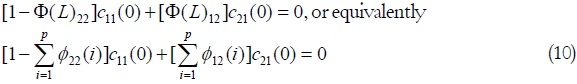
The parameters Φ_j2 in (10) can be estimated by a var regression. With the three equations given on (7), a system of nonlinear equations and variables is specified and can be numerically solved.⁴

 

UNIT ROOT, STRUCTURAL BREAK TESTS, AND EMPIRICAL RESULTS

The series was first tested using the augmented Dickey-Fuller tests. Thus, considering a general autoregressive process of order p for the variable z that is estimated with H₀, which assumes the existence of a unit root, corresponding to the case where γ = 0. In this case, the equation is entirely in first differences, and so it has a unit root.

The lag length (p*) was set following the procedure suggested by Campbell and Perron (1991, 153-5), which indicates the use of standard t-tests to determine it. The basic idea is to start with a supposedly large enough p and test against alternatives of fewer lags, stopping when the last lag is significantly different from zero.

The In Y product series was tested using (11) with p* = 2 and the hypothesis of a unit root was not rejected at the 5% level. On the other hand, it was rejected for its difference. Hence, the assumptions concerning Mexico's output process are similar to previous work done on Mexico's output dynamics, such as in Castillo and Díaz-Bautista (2003). Table 4 shows the basic results of the tests for output and output growth.

The results in Table 5 show the different dynamic nature of the labor market in Tijuana when compared to Mexico City. A comparison of those 2 cities shows different results for each in terms of stationarity using the Mexico City unemployment series and the Tijuana unemployment series. I examined the stationarity of a variable just by looking at the figure. Figure 1 shows the traditional open unemployment rate in Tijuana and Mexico City. Both unemployment series seem stationary. However, it is not obvious to the econometrician since the mean changes over time and there is no single trend. The ADF test indicates that unemployment series is integrated of order 1 for Mexico City.

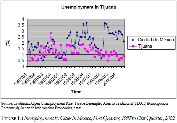
The unemployment series for the City of Tijuana is stationary and integrated of order 0. One explanation for the rejection of the unit root hypothesis in one of the cases could be these tests' widely recognized low power. This explanation is also supported by the results reported in other articles. For example, when testing unit roots for the U.S. economic series, unemployment is among those variables for which stationarity is most strongly accepted. This is the case in the famous articles of Nelson and Plosser (1982) and Alana and Robinson (1997), who use a test for unit roots (and nonstationarity in general) based on fractional roots as the alternative hypothesis. Nelson and Plosser, testing the same 14 variables they had previously used in that article, find again that unemployment is the closest to stationarity. The results of Song and Wu (1997) are also significant. Using unemployment data for 48 U.S. states, they show that the ADF test rejects H₀ for only three series (the Philips-Perron test rejects for one more state). However, using a panel-based test, the null is easily rejected, even when the data are not used for the four states that previously had H₀ rejected by at least one of the traditional tests.

Certainly, evidence against the stationarity of unemployment series can be found. Nevertheless, it is by now widely accepted that simple econometric unit root tests cannot be used as the only proof for the existence of stationarity or nonstationarity, especially for small samples. Thus, an agnostic view would suggest that we simply assume Tijuana's unemployment is stationary. An alternative procedure is to model the unemployment series including trend specifications. Such strategy is informally supported by its temporal pattern, which can be described as having an inverted U-shaped fluctuation.⁵ Thus, besides the original series, two other specifications were used, one with a quadratic trend, and another assuming two distinct linear trends (that is, imposing a structural change in the fourth quarter of 1994). Although the hypothesis of a structural change is here assumed without a formal theoretical justification, there are some facts that can justify it. The end of 1994 was a very significant year for the Mexican economy because of the start of the Mexican recession and the end of the Salinas administration. The change of presidential administrations traditionally signifies the breaking of employment contracts (usually accompanied by a large wealth redistribution from creditors to debtors) and changes in prices and wages for an undetermined period. Hence, an informal analysis of Mexico's macro-economic policies, with society's responses to it, suggests that a structural change in its trend is a possibility that should be considered in the unemployment series.

In order to test econometrically the existence of a unit root in the unemployment series, accounting for a structural change, the technique presented by Perron (1989) is used.⁶ It can be viewed as an extension of the adf procedure but one having distinct critical values:

where the three variables are such that SCP_t = 1 in the first quarter of 1987, SCL_t = 1 after the fourth quarter of 1994 and SCP_t = t after the fourth quarter of 1994; otherwise they are zero. H₀ assumes γ = β_t = β₁ = 0, while H₁ says γ < 0 and δ₀ = 0. The test is two-step: First, I regress u_t on (s, t, SCL, SCT), where s is the vector of constants; then, using the residuals of that regression, test if they have a unit root in the usual way. The critical values depend on when the change has occurred, that is, on the value λ = t*/T, where t* is the first period after the structural change and T is the number of observations.⁷ The first regression presents coefficients for scp and scl statistically very significant with an F-test for the constraint that they are both zero being easily rejected.

Besides that, the unit root test rejects the null hypothesis, as showed in Table 6.

The results further support the existence of a stationary series for Tijuana's unemployment even when structural breaks are considered. To further support the results, I used three different specifications for that variable: the original, the specification with a permanent change in the slope, and the specification assuming a structural change in the fourth quarter of 1994. As usual in VAR estimations, the regressors of both equations are the same. Hence, even though a SUR model applies, OLS estimation in each equation is consistent and asymptotically efficient. In order to determine the appropriate number of lags (p) in the system, two guides were used, leading to different specifications. First, I chose p = 8, assumed to be large enough to capture all economically significant serial correlations. Blanchard and Quah (1989) also chose this. To ascertain if the choice of a smaller p would be possible without any significant loss, I used the Akaike Information Criterion (AIC). It suggests the choice of p that makes the value AIC = T ln|Var(e_t) + 2N the smallest possible, where T = number of usable observations; |Var(e)| = determinant of the estimated variance matrix of the residuals; and N = number of estimated parameters in the system, here 2(2p+1). With all unemployment treatments, the indicated p was 3. A likelihood ratio test was also performed, in order to check the AIc results. Two alternatives were tested, with p = 4 and p = 2, given H₀: p = 3. The null hypothesis was easily accepted in all cases (considering each of the series used for unemployment), even at 10% of significance.⁸ Following the test, an autocorrelation test for the var with p = 3 was used. Using the Ljung-Box statistic, the hypothesis of white noise was always accepted at the 5% level of significance, confirming the appropriateness of that specification.⁹ Hence, all the performed tests suggested the choice of a 2 lags specification. As in Blanchard and Quah (1989), the analysis of the identification is twofold: first, determine the dynamic responses to each kind of disturbance, and second, measure the relative contribution of each for the two employed economic variables.

One general result from the analysis of the unemployment series of the estimated cases is a noticeable difference between the 1 and the 2 lags results, with the exception of the unemployment responses to demand disturbances. Generally, with 2 lags, the pattern in the short-run is less defined and the unemployment shocks need a longer time to reach their long-run values than the unemployment shocks calculated using only 1 lag. These differences are explained basically by the wider confidence intervals for the point estimates that come up when p=2 is used instead of p = 1, a feature generally obtained and that is especially significant when using the detrended series for unemployment. Generally, this result is a consequence of the estimations in the 2 lags case: Even though most of the parameters are not statistically different from zero, their absolute values are not necessarily small, often substantially affecting the unemployment-shock point estimates. This is an effect of the loss in degrees of freedom (two more parameters to be estimated in each equation) that a less parsimonious model might imply. The choice of the unemployment series used as a measure of unemployment also matters, even though only small differences appear between the two detrending procedures. Thus, the cases for two linear trends are not shown.

The U.S. responses to demand shocks in terms of output and unemployment (Blanchard and Quah 1989) are also seen for Tijuana. An exogenous transitory shock in demand is one that has a decrease in unemployment, where wage rigidity represents a simple explanation for cyclical unemployment as in Quandt and Rosen (1988). An exogenous shock in demand could come from a change in technology and marginal revenue product of labor, the demand for final products, and from the supply of complementary and anti-complementary inputs.

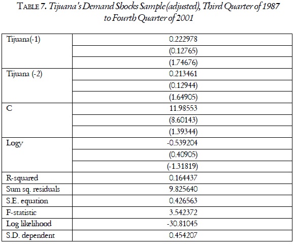
Table 7 presents the EViews econometric software output from Tijuana's Demand Shock sample between the third quarter of 1987 and the fourth quarter of 2001. The output is rather conventional in format. However, an interesting result is how Okun's Law differs from previous studies. Using the original log series, Okun's coefficient is 5.3, while the coefficient relation for industrialized countries averages about 2.5.¹⁰ We observe three features that are present in Okun's Law. First, the inverse relation between the increase in output growth that will cause reductions in unemployment. In Tijuana, in order to increase the economy's output, firms should increase employment, which causes unemployment to decrease. Second, the coefficient in Okun's Law is determined by the amount of labor hoarding in Tijuana's economy and also by the changes in labor-force participation as employment is changing. The third feature is that we assume a natural growth rate, as employment is growing at the same rate as the labor force.

Keynesians say that there are rigidities in the economy that are slow to adjust to equilibrium. Therefore, the natural unemployment rate is between 1% and 1.5%, which reflects the long-run equilibrium of the economy, and when an exogenous variable changes due to a demand shock, the adjustment from one equilibrium to another occurs at a moderate pace for output.

Output overshoots in the first five periods and later reaches its long-run level, while unemployment deviates from its natural rate and reaches a lower rate after 15 periods. Moreover, the lump-shaped effect appears in the response of output when the original series for unemployment is used, but even then, the lump is relatively small. For a demand shock, unemployment ends at a lower level after 10 to 15 periods, while output reaches the same natural rate after 20 to 25 periods (Figure 2).

With respect to the supply shocks, on the other hand, the impulse responses are quite similar regardless of the series used for unemployment. The EViews output for Tijuana's supply shock is in Table 8. The supply-shock model is significant with a positive permanent supply shock, with some short-run overshooting effects on output. Output reaches a higher level after 16 to 20 periods. Exogenous shocks to supply could originate from wealth effects, demography, amenities and standards of living, or even social forces and legislation. A famous example of a supply shock was the Black Death, which killed one third of the population in Europe between 1348 and 1350. In our case study, demographic effects in Tijuana could better explain the supply shocks. The initial response of unemployment after a positive supply shock is lower unemployment with a gradual return to the same level after 15 to 20 periods. Indeed, the impulse response function for Tijuana's unemployment does have a slight U shape through time.

The results suggest that the nominal rigidities observed in Tijuana are large compared with the United States, if they exist at all. Since we have nominal rigidities, with a positive supply shock (a productivity improvement), aggregated supply would be higher, but aggregated demand would react slowly. Consequently, while output monotonically increases, reaching its new equilibrium value, employment would initially fall because of the difference, where aggregate supply is greater than aggregate demand, returning to its long-run value only gradually, as the gap is being eliminated. The estimations with 2 lags display a pattern that could be consistent with nominal rigidities. With real rigidities, having real wages fixed, unemployment would decline, and output would jump up to above its new long-run equilibrium level. Then, we would expect the real wages to be adjusted, and the initial overreaction would be gradually eliminated. The estimates for Tijuana suggest that this may be the case, but only to a small extent, because of the convergence to the long-run values. A number of justifications could be given to explain those patterns. The most obvious may be the maintenance of very high inflation for the break period. Within that economic environment, the setting of real wages is certainly facilitated, thus justifying real rigidities.

The identification scheme provides us with the series of structural disturbances v_t so we can verify the variation of a given variable due to each kind of shock. Among them, the 1994 recession and the expansion at the end of the 1990s were essentially a consequence of internal policies, while the others were fundamentally driven by external factors (the oil and interest-rates crisis, the two Mexican crisis, and the beginning of the Asian meltdown). From the results, we can say that the 1995 recession was essentially a supply-driven shock, mainly demographic, while the other periods show no clear trend toward either demand or supply disturbance. We could say that demographics, social forces, legislation and regulation, wealth, technology, and demand for final products affect the dynamics of the labor market in Tijuana. By considering the special characteristics of each period, the results confirm economic intuition. The recession in the 1990s brought an increase in the price of oil and international interest rates. These movements suggest a once-and-for-all reduction in national output due to the uncertainty in the economic environment.

A final observation is that in the second quarter of 2000, the Tijuana labor market reached a steady state, that is, the unemployment rate was around 1.3%, or we can say that the number of people finding jobs was approximately equal to the people looking for jobs. Any policy in Tijuana aimed at further lowering the natural unemployment rate must reduce the rate of job separation or increase the rate of job finding.

 

CONCLUSION

This article used the time series structural break and var methodology to identify demand and supply shocks in Tijuana, Mexico. The Tijuana unemployment series contrasts significantly with previous results for the United States and the estimated results for Mexico City, with the roles of demand and supply disturbances varying greatly between Tijuana and Mexico City. The empirical results indicate that, provided the correctness of the identification, two distinct economies may react very differently to the same type of shock. The results for Tijuana shows that a positive supply shocks raises output in both the short and the long term, while unemployment returned to its original level after 37 periods.

At least two adjustment mechanisms may be present in Tijuana's unemployment, such as migration to the United States and the growth of the informal sector in Baja California. Thus, if someone is looking for a general macroeco-nomic theory, this is a disappointing fact, due to the distinct and different results in Tijuana when compared to Mexico City and the United States. Nevertheless, the identification restriction may not be appropriate. As the analysis of some special periods has suggested, it is possible that supply and demand innovations do have a non-zero correlation, perhaps reflecting policy reactions to exogenous disturbances.

The data analysis shows that Mexico has had a lower unemployment rate than the United States and the European Union (EU). Mexican unemployment is characterized by different dynamic trends than the industrialized countries. Over the last 15 years, Portugal and the United States have had the same average unemployment rate, about 6.5%, while Mexico's rate was less than half the rates in other oecd countries, showing very different labor markets. Unemployment in the EU began to escalate in 1991 and slowly rose to a maximum of 11.6% in 1994, as reported by Eurostat (2000). In 1996, 11.4% of all economically active Europeans were out of a job: Almost 19 million people were unemployed. Germany, France, Italy, Belgium, Finland, Greece, Ireland, Luxembourg, Spain, and Sweden almost doubled and, in some cases, even tripled their unemployment figures from the 1980s to the end of the 1990s. In Mexico, and in Tijuana, in particular, unemployment figures were stable during the 1980s and 1990s. Of the 15 EU member states, Portugal was the only one to register a drop in unemployment rates from the 1980s (8%) to 1996 (7.2%), all others showed dramatic increases over the same period. The oecd area unemployment rate on a standardized basis was 6.3% in April 2001, more than twice the Mexican unemployment rate. Mexico has adjusted its measures when necessary, and as far as available data allow, but it should update and bring the unemployment measures as close as possible to International Labor Organization, U.S. Bureau of Labor Statistics, and Eurostat guidelines for international comparisons of labor-force statistics. Further work in this area should compare the unemployment situation in Mexico with respect to North American Free Trade Agreement and EU member states.

 

REFERENCES

Alana, G. L., and P. M. Robinson, 1997, "Testing of Unit Root and Other Non-stationary Hypothesis in Macroeconomic Time Series." Journal of Econometrics 80:241-68.         [ Links ]

Blanchard Olivier Jean, and D. Quah, 1989, "The Dynamic Effects of Aggregate Demand and Supply Disturbances." The American Economic Review 79:655-73.         [ Links ]

Blanchard, Olivier Jean, and Lawrence F. Katz, 1992, Regional Evolutions, Brookings Papers on Economic Activity 1/1992. Available at http://www.brook.edu/dybdocroot/es/commentary/journals/bpea_macro/tocs.htm.         [ Links ]

Campbell, John Y., and Pierre Perron, 1991, "Pitfalls and Opportunities: What Macroeconomists Should Know about Unit Roots." NBER Macroeconomics Annual, Cambridge, Mass.: MIT Press.

Castillo, Ramón, and Alejandro Díaz-Bautista, 2003, "Testing for Unit Roots: Mexico's GDP," Working Paper, Department of Economic Studies, El Colegio de la Frontera Norte, forthcoming in review Momento económico.         [ Links ]

Christiano, Lawrence J., 1992, "Searching for Breaks in GNP," Journal of Business and Economic Statistics, 10:237-50.         [ Links ]

Enders, Walter, 1995, Applied Econometric Time Series, New York: John Wiley & Sons.         [ Links ]

Enders, Walter, and B. S. Lee, 1997, "Accounting for Real and Nominal Exchange Rate Movements in the Post-Bretton Woods Period," Journal of International Money and Finance, 16:233-54.         [ Links ]

Fleck, Susan, and Constance Sorrentino, 1994, "Employment and Unemployment in Mexico's Labor Force," Monthly Labor Review, 117 (11):3-31. Available at http://www.bls.gov/opub/mlr/1994/11/contents.htm.         [ Links ]

Gamber, E. N., 1996, "Empirical Estimates of the Short-Run Aggregate Supply and Demand Curves for the Post-War U.S. Economy," Southern Economic Journal, 62:856-72.         [ Links ]

Gamber, E.N. and F.L^®. Joutz, 1993, "An application of Estimating Structural Vector Autoregression Models with Long-run Restrictions," Journal of Macroeconomics, 15:723-45.         [ Links ]

Instituto Nacional de Estadística, Geografía e Informática, Statistics for various years. Available at: www.inegi.gob.mx.         [ Links ]

Nelson, C., and Plosser C., 1982, "Trends and Random Walks in Macroeconomics," Journal of Monetary Economics, 10:139-62.         [ Links ]

Perron, Pierre, 1989, "The Great Crash, the Oil Price Shock, and the Unit Root Hypothesis," Econometrica, 57:1361-1401.         [ Links ]

Quandt, Richard E., and Rosen, Harvey S. 1988. The Conflict between Equilibrium and Disequilibrium Theories: The Case of the U.S. Labor Market. Kalamazoo, Michigan: The Upjohn Institute.         [ Links ]

Revenga, Ana, and Riboud, Michelle, 1993, Unemployment in Mexico: Its Characteristics and Determinants, Report Number WPS1230, World Bank Policy Research Working Paper, Washington, D.C.         [ Links ]

Song, F. M., and Y. Wu, 1997, "Hysteresis in Unemployment: Evidence from 48 U.S. States," Economic Inquiry, 35:235-43.         [ Links ]

Statistical Office of the European Communities (Eurostat), 2000. Available at http://europa.eu.int/comm/eurostat/Public/datashop/print-catalogue/EN?catalogue=Eurostat.

U.S. Bureau of Labor Statistics, Local Area Unemployment Statistics Website. Available at http://www.bls.gov/lauhome.htm.

U.S. Department of Labor, Bureau of Labor Statistics, 2001, How the Government Measures Unemployment. Updated Version of Report 864 (July). http://www.bls.gov/cps/cps_htgm.htm.         [ Links ]

 

Notas

¹Article 303 of the North American Free Trade Agreement bars Mexico from lowering tariffs on inputs and primary materials when they are imported from countries that are not nafta members or when those materials are used in products that may later be exported to the United States or Canada. Maquiladora plants manufacturing products for export outside the nafta region will continue under a temporary import regime.

²"Frictional unemployment" is unemployment resulting from labor turnover; that is, since it takes time to find a job, flows in and out of the labor market create a pool of (temporarily) unemployed people. People who are between jobs are fictionally unemployed.

³Expression (7) comes directly from (3), after taking the variances in that equation.

⁴As Enders (1995, 353) points out, the system has "multiple" solutions, in the sense that some alternatives with the same absolute value but opposite signs are possible, because of the nonlinear terms. In fact, exactly four combinations are possible: Given that (c₁₁, c₁₂, c₂₁, c₂₂) is a solution, (c₁₁, -c₁₂, c₂₁, -c₂₂), (-c₁₁, c₁₂, -c₂₁, c₂₂), (-c₁₁, -c₁₂, -c₂₁, -c₂₂) are too, where the indices were dropped. As in the standard literature, the one used gives a positive response of Dy to positive demand and supply shocks, which consists of the (unique) case where c₁₁ and c₁₂ are both positive.

⁵The inverted, U-shaped fluctuation of the Tijuana unemployment series is further strengthened when the 2002 data is included, indicating the appropriateness of the trend specifications.

⁶Certainly, this original way of accounting for breaks in time series is open to the critique that the period chosen for the break point was selected in order to manipulate the results, since that choice is ad hoc.

⁷In the case studied here, λ=0.532. In Perron (1989), the critical values are tabulated for λ going from 0.1 to 0.9, with increments of 0.1. Thus, the values used are for λ=0.5, the most critical in the tables.

⁸The test-statistic is (T-c)(ln|Var(e_t)|_RESTRICTED-ln|Var(e_t)| _UNRESTRICTED), where c = number of estimated parameters in each equation of the unrestricted case, and it has an asymptotic x²(k) distribution, where k = number of restrictions in the system (Enders 1995, 313-315).

⁹The statistic is Q= T(T+2) Σr²_j /(T-j), with j from 1 to L, where r²_j is the j-th autocorrelation. The test was made for all L from 1 to 32. (See Greene, 1997, 595).

¹⁰Okun's Law summarizes the relation between output growth and change in unemployment. It indicates that when unemployment decreases 1 percentage point, output increases by 2% to 3% (and vice versa). This is because, when unemployment increases, output per hour worked falls due to labor hoarding, hours worked per employee falls, and the labor force contracts as workers become discouraged or take early retirement.