Introduction

As SARS-CoV-2 (COVID-19) spreads in Mexico, more characteristics of its transmission trends in individual states are becoming known. Determining the pattern of infections in space and time makes it possible to understand how the spread occurs and how it is transmitted amid the control measures established by epidemiological surveillance systems and, consequently, helps redefine intervention strategies to reduce the impact on the health of the population (^{Bhaskar et al., 2020}; ^{Cuartas et al., 2020}; ^{Medeiros et al., 2020}; ^{Parr, 2020}). This work aims to analyze the spatio-temporal pattern of the spread of COVID-19 in the municipalities of the border state of Baja California between epidemiological weeks 10 and 31 through the System Dynamics (SD) and Geographic Information Systems (GIS) methodologies. These tools can simulate the complexity and multiplicity of aspects involved in this type of epidemiological phenomenon (^{Castro et al., 2005}).

In order to model the critical factors of COVID-19 propagation, such as the rate of infection and the rate of recovery from infection, this work used the SIR epidemic model (^{Kermack & McKendrick, 1927}), which has been widely utilized in Mexico (^{Miramontes, 2020}; ^{Ortigoza et al., 2020}; ^{Ruiz, 2020}; ^{Vargas Magaña et al., 2020}). The information on cumulative confirmed cases per week comes from the General Directorate of Epidemiology of the Ministry of Health (Dirección General de Epidemiología de la Secretaría de Salud, DGE-SS) recorded on June 6, 2020.

On June 6, 2020, the State of Baja California surpassed the figure of 6 000 accumulated confirmed cases of COVID-19, ranking third in the country (^{DGE-SS, 2020}). The pattern of infections by municipality indicates that Mexicali is the main focus, with 3 079 ─half of the patients statewide─, Tijuana registered 2 276, Ensenada 312, Tecate 180, and Playas de Rosarito 64 (^{DGE-SS, 2020}). Tijuana leads the cumulative number of deaths from the disease with 643 deaths, followed by Mexicali with 495, Ensenada with 51, Tecate with 50, and Playas de Rosarito with 9. Additionally, it is important to highlight that this federal entity, when compared with national figures, has a state mortality rate of 2.36 per 100 000 inhabitants, well above the national average of 0.076 per 100 000 inhabitants, and a case fatality rate of 8.7%, which is also higher than the national average of 4.39% (^{DGE-SS, 2020}).

The results demonstrate that the epidemiological pattern tends to be spatially concentrated in Mexicali, Tijuana, and Tecate, cities that host cross-border workers between Baja California and California in the United States. In addition, the pattern reveals changing temporal trends in the municipalities of Ensenada and Playas de Rosarito, which are the most popular destinations with tourists visiting Baja California.

This work comprises seven sections. The first section presents a review of the literature on the spread of COVID-19 in Mexico. The second section presents the SIR model, which is called epidemic since the duration of the disease is short compared to the life expectancy of the host (^{Pérez, 2012}). The third section presents the SD methodology, useful for analyzing the structural causes that lead to the dynamic behavior of the SIR model, and the Stella software program, which is a tool that makes it possible to run numerical simulations of the SIR model on a computer. The fourth section presents the SIG methodology, useful for geographically representing the evolution of COVID-19 in the state. The fifth section presents the database. The sixth section discusses the results of the geographic-temporal evolution of COVID-19 transmission in the five municipalities of the border state of Baja California. Finally, the seventh section offers the conclusion.

Spread of COVID-19 in Mexico

In Mexico, the first confirmed case of COVID-19 was reported on February 27, 2020, of a person who traveled to Italy, and the first non-imported death from the virus occurred on March 19. By the first date, the country was in Phase 1, where confirmed cases of the virus in Mexico were associated with infected travelers from countries where the disease was present. In Mexico, between March 17 and 23, with the goal of reducing the number of contacts, the number and intensity of non-drug mitigation measures were increased. Among these measures were the cancellation of school activities, social distancing, hand washing, no kissing or hugging, and banning gatherings of more than 50 people. Two days later ─on March 25─ the declaration of Phase 2 was considered due to community infections in people with no history of travel abroad. A little less than a month later ─on April 21─ Mexico declared Phase 3, extending the Social Distancing Period and the suspension of activities until May 30 (^{Palacios, 2020}).

The SIR epidemic model, originally developed by ^{Kermack and McKendrick (1927}), has been applied in the country to determine when the outbreak of COVID-19 infection emerges, how it grows, and at what point it peaks and then declines (^{Miramontes, 2020}; ^{Ortigoza et al., 2020}; ^{Ruiz, 2020}; ^{Vargas Magaña et al., 2020}).

Thus, ^{Ruiz (2020}) simulated the infection based on the SIR epidemic model under certain assumptions: 1) The total number of people in the country is constant at 120 million, ignoring vital dynamics. 2) Any Mexican is susceptible to contracting the virus, except those who have recovered from the disease. 3) The spread of the virus in the country originated from a single person. 4) The virus has an infectious period of 14 days, corresponding to a daily recovery rate of infection γ= 14-1=0.072 days-1 and a daily infection rate of β=0.145 . 5) The initial conditions are: S0=0.99, I0=0.01. These data imply a reproduction rate of infection R0=2.2 .

From the simulation of the spread of COVID-19, the author concludes that, on average, each infected person was capable of infecting 2.2 people, that the maximum infected population would be 12%, and that after 365 days, the COVID-19 epidemic would end, counting from the first case on February 27, 2020.

Vargas Magaña and collaborators consider that, although the SIR model assumes the fixed β parameter during the evolution of the pandemic due to the application of anti-epidemic health policies in the country, it is possible to deduce that it tends to reduce its value temporarily. Consequently, it can also affect the basic reproduction rate of the infection over time. In this way, they analyze how epidemic mitigation measures affect the evolution of the average daily number of infected people β(t) over time, or alternatively, how the speed of infectious disease transmission was affected R(t) over time.

The authors point out that the Mexican health authorities implemented three sanitary phases, each one according to the degree of transmission of the disease. Each of these phases contributed to reducing the value of β and consequently to the decrease in the value of R0 from 2.409 to 1.391. Table 1 displays the mitigation or “flattening” effect of the initial outbreak of COVID-19 according to the following parameters β , γ, and R0 .

From the epidemic simulations, they infer that the decreasing growth of value R(t) is a sign of a successful flattening of the contagion curve, which in turn is the result of low mobility, isolation, suspension of certain economic activities, restriction of mass gatherings, and social distancing, among others. In the absence of a vaccine, the above measures were a solution to flatten the infection curve.

^{Miramontes (2020}) also analyzes the evolution of the number of infected people in different scenarios, where the difference is exclusively in the variation of the average daily infection transmission rate β(t ) and, therefore, in the uncertainty in the determination of the basic reproductive rate (R0 ). Miramontes establishes that several international studies indicate an average value of R0 = 3.28, but the uncertainty was high because the value of the coefficient ranged between 1.50 and 6.68 (Viceconte & Petrosillo, 2020 cited in ^{Miramontes, 2020}).

Finally, Ortigoza et al. numerically simulate an SIR epidemic model applied to COVID-19 for the state of Veracruz using weekly data. This simulation required fitting the SIR model to the official data utilizing parameter estimates γ and β with the use of a regression estimate between the officially infected subpopulation and the adjusted infected number from an initial SIR model. For the numerical simulation of the model, they used the Matlab 2017a package. A total population of 8 112 505 individuals was assumed with state-specific initial conditions of COVID-19 infection: S(0)=8 112 504 , I(0)=7 and R0=0 .

The results obtained for the parameters are γ=0.69 and β=1.33 . These parameters involve a ratio of R0=1.93 ; that is, each infected person could infect 1.93 people.

Figure 1 replicates the variation of the healthy, infected, and recovered populations involved in Veracruz when using the SIR epidemic model concerning time due to the systemic dynamics of the interactions between the populations.

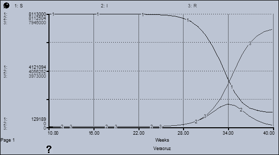
Source: Estimate by the author based on the parameters of ^{Ortigoza et al., 2020} Note: 1.S, healthy, 2.I, infected; and, 3.R, recovered

Figure 1 Progress of individuals that are healthy, infected, and recovered from COVID-19 in Veracruz 

The numerical simulation identifies that the maximum peak of infected people in Veracruz is reached in week 33.

In summary, the SIR epidemiological model has been applied in the country and states to understand the evolution and effect of COVID-19 containment measures.

Susceptible, infected, and recovered model (SIR)

The SIR epidemic model uses systems of differential equations coupled with certain elements of abstraction to describe, explain, and simulate the behavior of a disease that spreads by contagion in a population that remains constant. The model is also used as a decision-making tool to evaluate and define the best mitigation, prevention, or control strategy to limit a disease’s economic or health impact. Moreover, it serves as an analytical tool to improve the perception of the dynamics of contagious diseases, and thus validate the relationship of the predictor systems with the occurrence of the disease, mainly concerning the management of the basic reproduction ratio of the infection ( R0) that must be considered to control and eradicate the disease (^{García Piñera, 2014}).

^{Kermack and McKendrick (1927}) originally formulated the model based on the following postulates: 1) the disease can be viral or bacterial and is transmitted by direct person-to-person contact; 2) at the start of the epidemic, only a fraction of the population was infected; 3) the population is closed, and except for the few initially infected individuals, all others are susceptible to becoming ill; 4) the disease has a three-stage cycle: susceptible (S), infected (I) and recovered (R); 5) the patient undergoes the complete cycle of the disease and then recovers and acquires immunity; and, 6) the population is constant or without vital dynamics.

The following SIR epidemic model is considered epidemic because the duration of the disease is short compared to the life expectancy of the host (^{Pérez, 2012}). For this reason, births and deaths are not considered. The above means that the population is considered to be constant.

dSdt=- βSI [1]

dIdt= βSI-γI [2]

dRdt= γI [3]

Where the variations of the subgroups of the populations considered are described by the system of equations [1] to [3] and parameters β and γ denote the rates of infection and recovery, respectively.

Starting from the initial number of infected I(0) the initial population conditions required in the model are as follows,

N= S(0)- I(0) , I0 = I0 , and R(0)=0 In the epidemic model, the basic reproduction number is defined as ( R0) :

R0=βγ [4]

Thus the value of R0 will depend on the epidemiological characteristics of the disease as reflected by the parameters β , γ, and by the total population N. Therefore, R0 will take a constant value (^{García Piñera, 2014}).

The importance of parameter R0 lies in the fact that it can be used to determine whether there is an epidemic outbreak when a qualitative analysis of the previous models is carried out, noting that if

R0 >1 [5]

there will be an epidemic outbreak, and if

R0 < 1 [6]

there will not be an epidemic outbreak

In practice, one way to obtain information about β , γ, and R0 is to numerically simulate it over time through SD.

System Dynamics methodology

One of the approaches to obtain critical information from the model above is to simulate it numerically over time using the SD method to understand the structural causes that lead to the behavior of each system. The above involves increasing knowledge about the role of each element of the system and seeing how different procedures, performed on parts of the system, accentuate or attenuate the behavioral tendencies implicit in each one (^{Delgado, 2017}).

In order to gain knowledge of the structural causes that lead to the behavior of the systems, the SD methodology was based on the resolution of differential equations. The above was done with a structure based on the breakdown of these equations into types of variables, stock or state, flow or transfer, and auxiliary variables that make it possible to store formulas or parameters, and arcs representing the causal links.

Specifically, this work utilized Stella software as a visual modeling tool to conceptualize, document, simulate, analyze, and optimize system dynamics models. The Stella software program provides a simple and flexible way to build simulation models based on Forrester diagrams or stock and flow diagrams. The diagram elements are presented in Figure 2.

Source: ^{Forrester, 1960}

Figure 2 Elements of the Forrester diagram 

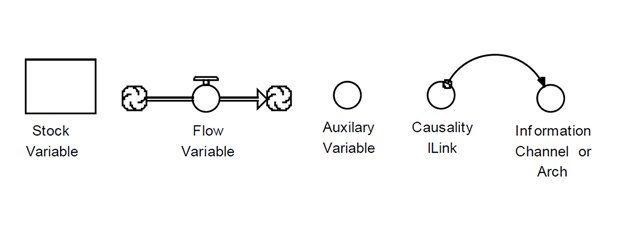
Thus, the set of variables of the models seen is transformed into the following:

Susceptible (status variable) representing the total population that does not have biological defenses to ward off disease contagion.

Infected (status variable) includes contagious patients not controlled by health services.

Recovered or deceased (status variable), which are patients who have been cured, become immunized, or died.

New infections (flow variable) denoting infection rate.

New cures (flow variable) indicating recovery rate.

Figure 3 depicts the SIR epidemic model in the Forrester flowchart.

Source: created by the author

Figure 3 Forrester flowchart for SIR epidemic model 

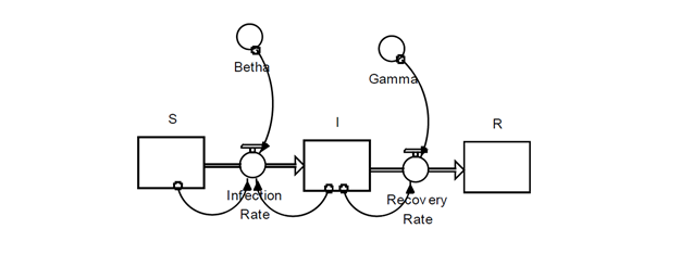
The Forrester diagram reveals that the variable of new infections is an accumulator. For each new interaction, the healthy individuals that became infected plus the infected from the previous interaction are added. The new cures variable is an accumulator of the infected that recovered. Stock data are stored in the variables susceptible or healthy stock (S), infected (I), and recovered (R). Thus, a cumulative number of infected can result from either a healthy or an infected stock in the previous interaction.

As a result of the simulation, the variation of the healthy, infected, and recovered populations involved in the model over time will be obtained due to the SD of the interactions between the variables of each model.

Geographic Information Systems (SIG) methodology

The model mentioned above and the distribution of several spatially distributed populations can be used to implement and run the GIS tool to visualize and interpret the fluctuations of healthy, infected, and recovered populations per polygon in an area of influence (^{Castro et al., 2005}).

The adjustment of the epidemic model in the GIS allows quantitative analysis of the spatial distribution by polygons, spatial correlation analysis of data, and studies of epidemic spread by geographical methods.

The specific methodology requires maps of the polygons of the region containing the tabular and spatial information of the healthy, infected, and recovered populations per polygon at an initial time. Then the initial maps are reclassified, which implies a) implementing the SIR model in the spatial data table; b) adjusting the range of variation of the previous populations of each polygon; and c) using the spatial analysis module of the GIS, classifying the data in intervals of equal magnitude in such a way that they can be visualized in a standardized way and making comparative analyses of the maps obtained. Furthermore, after the reclassification, the model can be run using the GIS platform for 20 interactions.

As a result, it is possible to present the initial distribution and the variation of infected persons by polygon in the area of influence of the COVID-19 pandemic in the municipalities of Baja California.

Database

The analysis of the evolution of COVID-19 was performed by Baja California municipality and for the California border counties during epidemiological weeks 10 to 31 of 2020. Daily data were obtained from the General Directorate of Epidemiology of the Ministry of Health (DGE-SS) for municipalities in Mexico and from USAFacts.org for counties in California. Once the daily information base was obtained, the weekly number of infected persons was created, as shown in Table 2 below.

Information is added for the counties of San Diego and the Imperial Valley in California, United States, due to their proximity and high levels of interaction in labor and economic terms with the municipalities of Baja California.

Temporal and spatial distribution of COVID-19 in Baja California municipalities

In order to illustrate the temporal fit of the SIR epidemic model applied to COVID-19 for Mexicali, Tijuana, Tecate, Ensenada, and Playas de Rosarito, this work used weekly data available on the number of COVID-19 infections from epidemiological week 11 to 31. The process of obtaining the parameter values β and γ required fitting an initial SIR model with the assumption of a contagion rate of 1.33 and a recovery rate of 0.39 (^{Ortigoza et al., 2020}). Subsequently, the residual sum of squares between the official number of confirmed infected persons and the number of infected persons was minimized from the adjusted SIR model (^{Ortigoza et al., 2020}).

Table 3 presents the results obtained for the values of β, γ and R0 for each of the municipalities in Baja California.

Table 3 presents the critical factors of the initial spread of municipal COVID-19 according to the model during epidemiological weeks 10 to 31, 2020. From the results, it can be seen that Mexicali shows the highest rate of contagion β = 1.60, while Tijuana presents the lowest recovery rate γ=0.59 . In addition, Mexicali displays an infection reproduction ratio of R0=2.46, which is higher than the national rate, which varies between R0=1.3 and R0=2.4 .

Figure 4 presents the simulations of the number of COVID-19 susceptible (1.S), infected (2.I), and recovered (3.R) individuals for Mexicali, which is the municipality with the greatest contact (for reasons of space, the others are not presented).

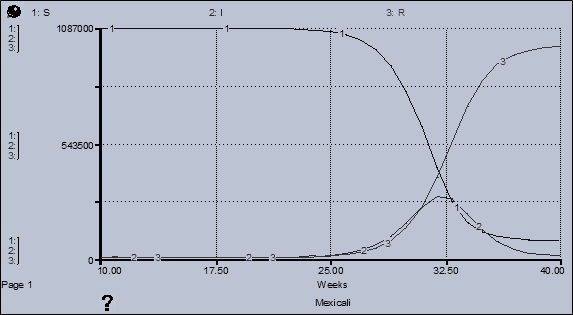
Source: created by the author Note: 1.S, healthy, 2.I, infected, and 3.R, recovered

Figure 4 Progress of individuals that are healthy, infected, and recovered from COVID-19 in Mexicali 

Figure 4 displays typical infection curves in which the peak of infection occurs around week 31 for Mexicali.

On the other hand, the analysis of infections from a spatial perspective makes it possible to know the location and incorporate the relationships between infections in one location relative to infections in other locations. This section provides a rationale to explain the behavior of the pandemic based on the interaction of residents of Baja California municipalities with San Diego and Imperial Valley counties in California, United States.

The following series of maps reveals the beginning of the pandemic and how its spatial distribution with the highest number of confirmed cases per week was in San Diego County. This county exhibited an initial growth during the first five weeks, then a 10-week period of stable behavior, and toward the end, after an accelerated growth for five weeks, a slight decrease in the final two weeks. Concerning the above, Tijuana, Tecate, and Playas de Rosarito ─geographically the closest to San Diego─ also display growth in the first weeks. However, this growth is observed until week 17, followed by five weeks, where it decreases and ends with sustained growth. In Ensenada, with significant tourist interaction with San Diego and the rest of the coastal corridor that includes Tijuana and Rosarito, there is sustained growth during the first 15 weeks and then a stable trend.

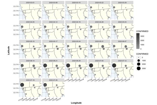
Source: created by the author based on statistics from the ^{DGE-SS (2020)} and from ^{USAFacts.org (2020)}

Figure 5 Spatio-temporal trends of COVID-19 in the border region of Baja California, Mexico, and California, United States 

Figure 5 demonstrates that, to the west of the study region, where the municipality of Mexicali and the county of Imperial are located, confirmed cases during the first ten weeks are more notable in the Baja California municipality. However, the Californian county has a very accelerated growth that reaches the same magnitude three weeks later and the following week surpasses Mexicali in the number of cases. In the final seven weeks, there has been a decrease in cases in both cities.

The temporal trends can be better appreciated in Figure 6 and Figure 7 for the San Diego-Ensenada and San Diego-Mexicali corridor, where the infection rates per 100,000 inhabitants are displayed, which, being related to the population, allow for comparability.

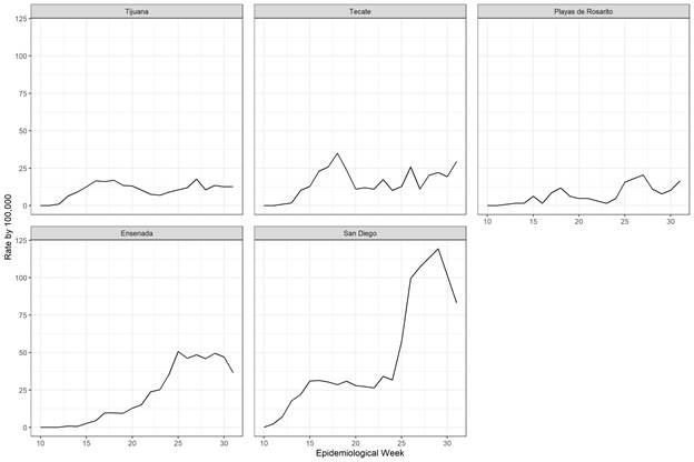
Source: created by the author based on statistics from the ^{DGE-SS (2020)} and from ^{USAFacts.org (2020)}

Figure 6 Temporal trends of the infection rate in the San Diego-Ensenada corridor 

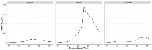
Source: created by the author based on statistics from the ^{DGE-SS (2020)} and from ^{USAFacts.org (2020)}

Figure 7 Temporal trends of the infection rate in the San Diego-Mexicali corridor 

The above interrelationships are supported by the correlation coefficient of the observed values. Figure 8 presents a block of significant correlations in which the first line is also included. This block is made up of Tijuana, San Diego, Ensenada, Playas de Rosarito and Tecate, where the strongest relationships are San Diego-Ensenada, San Diego-Playas de Rosarito and Tijuana-Tecate. However, spatial relations imply that access from San Diego to the tourist corridor is through Tijuana.

In addition, there is also another block on the left of the figure formed by Mexicali, Imperial, San Diego, Ensenada, and Playas de Rosarito, since the road infrastructure between Mexicali and Ensenada or Playas de Rosarito may represent an important barrier in the conception of the spatial relationship between them. Considering the above, the interrelationship may be limited to the local Mexicali-Imperial area, which may even include San Diego due to the size and diversity of its economy.

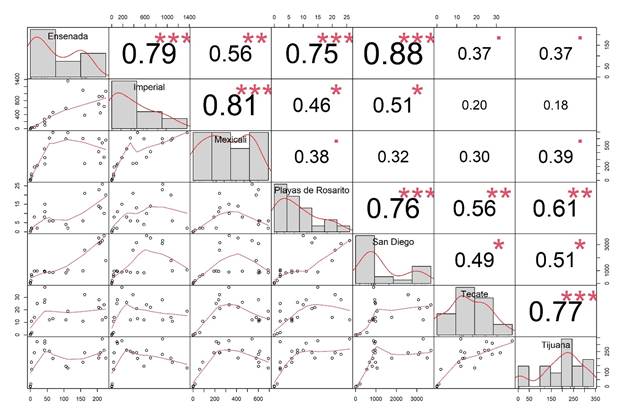
Source: created by the author based on statistics from the ^{DGE-SS (2020)} and from ^{USAFacts.org (2020)}

Figure 8 Correlation coefficients of confirmed cases per week 

The arguments put forward are based on the well-known first law of geography, which states that everything is related to everything else, but near things are more related than distant things. Considering this, the spatio-temporal relationship of COVID propagation in the study area can be visualized by using an interpolation by the inverse distance weighting method (IDW), which assumes that the similarities between the values of the points on a surface and the correlation rate between them are inversely proportional to the distance. The results for the number of confirmed cases in weeks 20, 25, and 31, displayed in Figure 9, indicate that San Diego has the highest number of cases at all times and that, in addition, it has an upward trend, which, due to its magnitude, is relatively independent. In week 20, Mexicali and Imperial present an associated trend that becomes dominated by the increase in Imperial and is less visible toward the end of the period analyzed. In the cases of Tijuana, Tecate, Playas de Rosarito, and Ensenada, week 20 presents differentiated trends with higher values in Tijuana that by week 25 have an appearance of associated trends and are different from the rest; toward the end of the period, what stands out the most are the differences in the trends of the Baja California municipalities compared with the California counties.

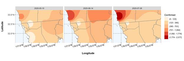
Source: created by the author based on statistics from the ^{DGE-SS (2020)} and ^{USAFacts.org (2020)}

Figure 9 IDW interpolation of confirmed cases in the study area 

When considering a similar analysis for the infection rate per 100,000 inhabitants, the similarity of the values for Tijuana, San Diego, Tecate, Playas de Rosarito, Ensenada, Mexicali, and the Imperial Valley is notable. However, the latter are impacted differently given the accelerated growth of the rate in the Imperial Valley compared to the variation in Mexicali. Although this growth decreases significantly at the end of the weeks studied, the above cases still maintain a relative difference (Figure 10).

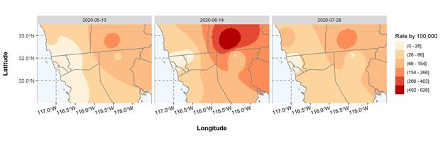
Source: created by the author based on statistics from the ^{DGE-SS (2020)} and from ^{USAFacts.org (2020)}

Figure 10 IDW interpolation of the infection rate in the study area 

In summary, a spatial pattern is confirmed that tends to be centralized in Mexicali and Tijuana. Cross-border workers who daily cross the international line to work in one of the California counties reside in these municipalities. There is a changing seasonal trend for Ensenada and Playas de Rosarito, the destinations of most Californian tourists who travel the tourist route of the coastal corridor that goes from Ensenada to Tecate and crosses the wine valleys in search of the beaches of Playas de Rosarito.

Conclusions

Regarding the temporal epidemiological pattern of Baja California, the municipalities of Mexicali and Tijuana stand out as the main centers of contagion, with displacement to Ensenada, Playas de Rosarito, and Tecate. This pattern of infection initially demonstrates that imported cases occur in Baja California municipalities that are home to cross-border workers who cross the border to work in San Diego and Imperial Valley counties in California daily. Subsequently, the contagions move to Ensenada, Playas de Rosarito, and Tecate, which are the destinations of most Californian tourists who travel along the tourist route of the coastal corridor. The above has implications for how the epidemic has been managed and differentiated costs for the inhabitants of Baja California.

The epidemiological pattern is influenced by the border transit of cross-border workers with dual nationality that is guaranteed by the uncontrolled crossing between countries, even when they may be infected. Moreover, U.S. tourists throughout this period were welcome to visit the tourist attractions of the Baja California coastal corridor, even when the number of infections was almost eight times higher than that of the municipalities on the Mexican side. Meanwhile, Baja California residents were limited to transit to California only for essential activities, as if the pandemic were occurring only on the Baja California side of the border.

Therefore, there is a need for health authorities to intervene to control the epidemic, not only by focusing on the immediate detection of autochthonous cases but also by improving the identification of imported cases in order to mitigate the spread of the virus in the state, as well as international agreements on sanitary controls so that there is no unequal treatment between citizens of one country and another.

REFERENCES

Bhaskar, A., Ponnuraja, C., Srinivasan, R. & Padmanaban, S. (2020). Distribution and growth rate of COVID-19 outbreak in Tamil Nadu: A log-linear regression approach. Indian Journal of Public Health, 64(6), 188-191. https://doi.org/10.4103/ijph.ijph_502_20 [ Links ]
Castro, C. A., Lodoño, L. A. & Valdés, J. C. (2005). Modelación y simulación computacional usando sistemas de información geográfica con dinámica de sistemas a fenómenos epidemiológicos. Revista Facultad de Ingeniería Universidad de Antioquia, (34), 86-100. https://www.redalyc.org/articulo.oa?id=43003408 [ Links ]
Cuartas, D., Arango-Londoño, D., Guzmán-Escarria, G., Muñoz, E., Caicedo, D., Ortega, D., Fandiño-Losada, A., Mena, J., Torres, M., Barrera, L. & Méndez, F. (2020). Análisis espacio temporal del SARS-COV-2 en Cali, Colombia. Revista Salud Publica, 22(2), 1-6. https://doi.org/10.15446/rsap.v22n2.86431 [ Links ]
Delgado, J. A. (2017). Dinámica de sistemas aplicado a la epidemiología. Seminario permanente: las matemáticas aplicadas a la epidemiología. Facultad de Matemática. UMC. Colombia. http://www.mat.ucm.es/~aramosol/TextoDeConferencia-JoseAlfonsoDelgado.pdf [ Links ]
Dirección General de Epidemiología de la Secretaría de Salud (DGE-SS). (2020). Bases de datos COVID 19 en México. https://www.gob.mx/salud/documentos/datos-abiertos-152127 [ Links ]
Forrester, J. W. (1960). The impact of feedback control concepts on the management sciences. Foundation for Instrumentation Education and Research. [ Links ]
García Piñera, A. (2014). Modelos de ecuaciones diferenciales para la propagación de enfermedades infecciosas (trabajo de grado). Facultad de Ciencias. Universidad de Cantabria, España. https://repositorio.unican.es/xmlui/bitstream/handle/10902/7125/Andrea%20Garcia%20Pi%C3%B1era.pdf?sequence=1&isAllowed=y [ Links ]
Kermack, W. O. & McKendrick, A. G. (1927). A contribution to the mathematical theory of epidemics. Proceedings of the royal society of London. Series A, Containing papers of a mathematical and physical character, 115(772), 700-721. http://links.jstor.org/sici?sici=0950-1207%2819270801%29115%3A772%3C700%3AACTTMT%3E2.0.CO%3B2-Z [ Links ]
Medeiros, A., Daponte, A., Moreira, D., Gil-García, E. & Kalache, A. (2020). Letalidad del COVID-19: Ausencia de patrón epidemiológico. Gaceta Sanitaria. Artículo en prensa. https://doi.org/10.1016/j.gaceta.2020.04.001 [ Links ]
Miramontes, O. (2020). Entendamos el COVID-19 en México. COVID-19 en México. http://scifunam.fisica.unam.mx/mir/corona19/ [ Links ]
Ortigoza, G., Lorandi, A. & Neri, I. (2020). Simulación numérica y modelación matemática de la propagación del COVID-19 en el estado de Veracruz. Revista Mexicana de Medicina Forense y Ciencias de la Salud, 5(3), 21-37. https://www.medigraphic.com/cgi-bin/new/resumen.cgi?IDARTICULO=94909 [ Links ]
Palacios, B. (2020). Breve cronología de la pandemia 28 de febrero/14 de septiembre de 2020. Ibero, 70. http://revistas.ibero.mx/ibero/uploads/volumenes/55/pdf/breve-cronologia-de-la-pandemia.pdf [ Links ]
Parr, J. (2020, 5 de mayo). COVID-19 data analysis, part 5: different models of infection rates in Mexico and what they tell us. Digital@DAI. https://dai-global-digital.com/covid-19-part-5-different-methods-to-model-infection-rates-in-mexico-and-what-they-tell-us.html [ Links ]
Pérez, V. (2012). Estrategia de vacunación para una epidemia de influenza (Tesis de maestría). CIMAT, México. [ Links ]
Ruiz, V. R. (2020). COVID-19 México, modelo matemático revela que sistema sanitario de México estará rebasado entre mayo y junio. Revista Contra Línea. https://contralinea.com.mx/covid-19-modelo-matematico-revela-que-sistema-sanitario-de-mexico-estara-rebasado-entre-mayo-y-junio/ [ Links ]
USAFacts.org (2020). US COVID-19 cases and deaths by state. https://usafacts.org/visualizations/coronavirus-covid-19-spread-map [ Links ]
Vargas Magaña, R. M., Vargas Magaña, M. & Fromenteau, S. (2020). Impacto de las medidas de control en la evolución del brote COVID-19. En colaboración con el Colectivo Científicos Mexicanos en el Extranjero. https://mexiciencia.github.io/y Laboratorio ConCiencia Social https://concienciasocialla.wixsite.com/misitio [ Links ]
Alejandro Brugués Rodríguez Mexican, born in Havana, Cuba. PhD in Economics from the Universidad Autónoma de Baja California. Professor-researcher at the Department of Economic Studies of El Colegio de la Frontera Norte. Member of the SNI level I. Research lines: regional studies and economic development. Recent publication: Fuentes, N. A., Brugués, A. & Carrillo, J. (2020). Impacto económico de la reducción de la tasa del IVA en la región fronteriza norte de México con base en el uso de precios implícitos en el modelo insumo-producto. Revista de economía, 37(95).
Noé Arón Fuentes Flores Doctor of Economics, University of California, Irvine. Research professor at the Department of Economic Studies of El Colegio de la Frontera Norte. Member of the SNI level II. Research lines: regional development, border economy and Input-Output models. Recent publication: Fuentes, N. A., Brugués, A., González, G. & Carrillo, J. (2020). El impacto económico en la industria maquiladora y en la región fronteriza del norte de México debido al alza de 100% del salario mínimo. Región y sociedad, 32.
Received: October 05, 2020; Accepted: May 25, 2021
Este es un artículo publicado en acceso abierto bajo una licencia Creative Commons