nueva página del texto (beta)
 Inglés (pdf)
 Artículo en XML
 Referencias del artículo
 Enviar artículo por email
 Citado por SciELO
  Similares en
SciELO
Similares en
SciELO 
 Permalink
1. Introduction
In recent years, wind energy has become a renewable energy source increasingly developed worldwide, motivated by its cost-effectiveness and the need to explore new sources that limit greenhouse gas emissions. In Mexico, wind technologies have been gradually incorporated into the national energy generation system, achieving significant results in many regions of the country (Hernández-Gálvez et al., 2019). By the year 2021, the installed capacity for wind power generation was 7154 MW, which produce 21.14 TWh per year (AMEE, 2022). The increasing development of wind energy in Mexico has been driven by environmental and socioeconomic factors, such as the urgency to reduce emissions, the capacity to create new jobs, and the economic benefits for rural areas where the farms are located.
As the wind power capacity increases, accurate forecast systems are increasingly required to integrate wind resources into the grid more efficiently and reliably (Kosovic et al., 2020), which reduces costs and allows operators to make better real-time and day-ahead decisions (Marjanovic et al., 2014). To this end, it is essential to have skillful short-term wind forecasts. However, the representation of the wind field by numerical weather prediction (NWP) models is challenging because they depend on microscale processes such as buoyancy and turbulent diffusion effects, which drive rapid changes in wind intensity (Flores et al., 2013; Prósper et al., 2019).
The problem of short to medium-term wind resources forecasting has been addressed earlier by means of physical, statistical, and hybrid models. Statistical methods usually employ historical wind power production data and meteorological variables, applying univariate models to predict future wind power values. Such methods can make use of either statistical or artificial intelligence models. Some examples of recent work can be found in Damousis et al. (2004), Fan et al. (2009), Chitsaz et al. (2015), Osório et al. (2015), Heinermann and Kramer (2016), Dowell and Pinson (2016), Azimi et al. (2016), Zhao et al. (2016), Yuan et al. (2017), Chang et al. (2017), Liu et al. (2017), Naik et al. (2018), Valldecabres et al. (2018), and Hao and Tian (2019). Physical approaches are mainly based on NWP model results to obtain an estimate of the local wind speed forecast (Cassola and Burlando, 2012). Some relevant examples are Pinson et al. (2009), Khalid and Savkin (2012), and Prósper et al. (2019). Hybrid methods that combine NWP and statistical approaches are also found in previous literature; in these cases, NWP forecasts are coupled with statistical methods to obtain a wind power prediction for a turbine or a farm. Such methods can include bias correction techniques, ensemble forecasting, or artificial intelligence techniques. Among the most relevant are Louka et al. (2008), Cassola and Burlando (2012), Che et al. (2016), Che and Xiao (2016), Li et al. (2016), Zhao et al. (2017), Andrade and Bessa (2017), and Gilbert et al. (2020). In general, statistical methods are adequate for very short (a few seconds to 30 min ahead) and short-term (30 min to 6 h ahead) forecasts, while NWP and hybrid methods can be employed for longer-term forecasts, from hours to days ahead (Sweeney et al., 2020). Combined approaches are needed to obtain an advanced forecasting method with higher precision levels and longer forecast horizons, particularly for sites with complex terrain. In fact, hybrid methods generally outperform individual models (Tascikaraoglu and Uzunoglu, 2014; Okumus and Dinler, 2016; Méndez-Gordillo et al., 2022). In particular, hybrid methods that use NWP tend to outperform statistical approaches after a lead time of 3-6 h, therefore, they are present in most operational and commercial uses (Giebel and Kariniotakis, 2017).
In Mexico, some progress has been made on wind speed and wind energy forecasting methods, the most relevant are summarized below. Cadenas and Rivera (2007) implemented two time-series models to produce monthly wind speed forecasts for a wind farm in Oaxaca (southwestern Mexico). The same authors then applied an artificial neural network (Cadenas and Rivera, 2009) and a hybrid (autoregressive integrated moving average and ANN) method (Cadenas and Rivera, 2010) to hourly time series, obtaining accurate forecasts for short-term wind speed. Rodríguez-García et al. (2008) presented a short-term forecast method based on several statistical approaches. Cadenas et al. (2010) employed a single exponential smoothing method to forecast wind speeds in Chetumal, in eastern Mexico. Ibargüengoytia et al. (2014) developed a dynamic Bayesian network model based on historical time series for wind velocity prediction at a wind farm in Oaxaca, Mexico, for a short-term forecast horizon of 5 h. Méndez-Gordillo et al. (2022) proposed a hybrid statistical technique that includes a separation of turbulent and non-turbulent flows to forecast wind speed one step ahead at two sites in the northern Gulf of Mexico. Also, Santamaría-Bonfil et al. (2016)) employed a hybrid statistical approach based on support vector regression, obtaining accurate results for medium to short-term wind speed and power forecasts in southwestern Mexico. None of these previous works have made use of the advantages of NWP to forecast wind-power-related variables, in order to expand the forecast horizon of wind energy.
In this study, a combined framework for medium-term wind energy forecasts (24-h ahead) is developed and evaluated, integrating NWP and machine learning. The forecast system is implemented in a total of 41 wind farms throughout Mexico. However, since most of the farms have privacy regulations for the data generated at the farm, we show in this paper the results for only one wind farm located on the peninsula of Baja California. Our main objective is to assess the functionality of the proposed methodology and to evaluate its performance under strong synoptic forcing conditions. This framework is ideally useful for several applications, from electricity companies to wind farm developers, and it is also relevant to scientific applications regarding the use of combined methods for wind energy forecasting. To our knowledge, a hybrid approach to wind power forecasting like the one proposed in the present manuscript has not been applied before to wind farms in Mexico, a region where wind power prediction becomes difficult because of the complex topography and dynamic aspects of the weather patterns.
2. Methods
2.1 Measurement site and data processing
This study is based on data measured and collected at La Rumorosa wind power plant, located in the municipality of Tecate in the state of Baja California, northwestern Mexico. Figure 1 shows the location of the plant and the topography of the region. La Rumorosa is located at the northern end of the Baja California peninsula, at an altitude of around 1350 masl. The power plant has a total of five wind turbines (Fig. S1b in the supplementary material) with a nominal power output of 2000 kW (CEEBC, 2022), which gives a combined maximum production capacity of 10 000 kW. The turbines are located at a distance of nearly 200 m from each other; thus, the total extension of the park is less than 1 km. They are oriented in a north-northwest to south-southwest direction, and the predominant wind direction (coming from the west-southwest) is nearly perpendicular to the turbine distribution.

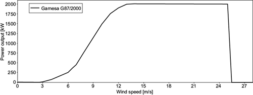
The La Rumorosa wind farm is made up of five Gamesa G87/2000 wind turbines with a rotor diameter of 87 m and a hub height of 78 m above surface level. Figure S2 in the supplementary material shows the power curve of the Gamesa turbine, which starts producing electric power at a wind speed of 3 m s−1, reaching its nominal power at 14 m s−1. The survival wind speed is 25 m s−1, which is the cutoff wind speed for power production.
Data from the La Rumorosa wind farm consists of 10-min wind power time series for each wind turbine, and wind speed and direction measured by anemometers at each turbine for 2015, 2016, and 2017. All datasets are processed to obtain hourly averaged values. A turbine nacelle-averaged wind hourly data for the entire site is constructed by averaging data from the five turbines. The nacelle-averaged values can be considered representative of the whole plant because the turbines are arranged along a line and the wake effects are negligible. Statistical analysis of the time series of wind speed and direction for all the turbines showed that they are comparable, exhibiting a high correspondence among them. This is evident by correlations above 0.97 for wind speed and above 0.85 for wind direction (Figs. S3 and S4 in the supplementary material). For constructing the wind power time series for the site, the values in all turbines are added, obtaining a total power generation for the farm.
2.2 Numerical simulations
Numerical simulations were performed to obtain modeled meteorological data for the period 2015-2017 at the site of interest, using the Weather Research and Forecasting (WRF) model. WRF is a NWP model supporting atmospheric research and weather forecasting. The Advanced Research WRF (ARW) core uses a non-hydrostatic approximation, with a horizontal staggered Arakawa C grid and terrain-following vertical coordinates near the surface. The WRF model has a range of physical options to parameterize and represent microphysical processes, cumulus convection, surface layer, boundary layer, and radiation (Skamarock et al., 2008). This research employs the ARW core, with four one-way nested domains (Fig. 2), centered on La Rumorosa site. The horizontal spacing from the outermost (Domain 1: D01) to the innermost (Domain 4: D04) domains are 75, 15, 3, and 1 km, respectively. The corresponding number of grid points are 56 × 56, 81 × 81, 96 × 96, and 178 × 163. The innermost domain is employed to extract a time series of meteorological variables corresponding to the site of interest. Finally, the NCEP-FNL Operational Global Analysis (NCAR, 2000) at 1º horizontal resolution is used as input for initial and boundary conditions, and the set of parameterizations are listed in Table I.

Fig. 2 Configuration of four nested domains for WRF simulations. Horizontal resolutions for D01, D02, D03, and D04 are 75, 15, 3, and 1 km, respectively.
Table I WRF parameterizations used in the present work.
| Physic option | Scheme used |
| Radiation-shortwave | Dudhia |
| Radiation-longwave | RRTM |
| Microphysics | Lin (Purdue) |
| Cumulus | Kain-Fritsch |
| Boundary layer | YSU |
| Surface layer | MM5 similarity |
| Land surface | Noah Land Surface Model |
Simulations are restarted every 30 h, taking the first 6 h as spin-up and keeping a complete diurnal cycle of 24-hourly values. In this way, the entire dataset of WRF simulations for 2015-2017 is built, containing the following variables: horizontal components of wind (u, v), temperature, and relative humidity, interpolated to rotor height.
2.3 Three-dimensional variational data assimilation for bias correction
In the present work, the output of WRF is post-processed to correct the biases that are intrinsically present in NWP models. The three-dimensional variational data assimilation (3DVAR) method is used for this purpose. Despite the fact that the 3DVAR method is designed for data assimilation, here it is used to reduce the bias of the WRF model. The 3DVAR aims to obtain an optimal estimate of the actual atmospheric state through iterative minimization of the following cost function:
The solution of this equation represents a statistically optimal analysis of u given the two sources of information from the background u b and the actual measurement w. The first term, scaled by the error covariance B, aims to incorporate the departure of the analysis from the background. The second term, scaled by the error covariance R, considers the departure of the actual measurement w and Hu, which is the observation operator that maps the variables from model space to observation space. The second term aims to incorporate the prior information, scaled by the inverse of the covariance matrix (Lewis et al., 2006; Ahmed et al., 2020).
The minimizer of the cost function (Eq. 1) is
where d ob = w − Hu b is the innovation, K = BH T Γ−1 is the Kalman Gain, and Γ = HBH T + R is the total error covariance (Kabir et al., 2019). In this paper, we have focused on the bias correction of WRF wind speed only. The observed variable is thus the wind speed. The observational error covariance matrix R and the background covariance matrix B were estimated from three years of measurements and the WRF model output, respectively.
2.4 Neural network model
Artificial neural networks (NNs) have been proven to be efficient techniques for forecasting wind power due to their capabilities, such as self-learning, easy implementation, and establishing non-linear relationships between input and output datasets with a high degree of accuracy (Tascikaraoglu and Uzunoglu, 2014). In this work, a multi-layer perceptron (MLP) is used to model the relationship between WRF output and wind power generation. An MLP is a supervised learning algorithm that consists of multiple layers of neurons, including an input, an output, and several intermediate or hidden layers. The input layer receives the inputs (i.e., the features) and the output layer produces the output (i.e., the prediction). Each node in the intermediate layers applies a weighted sum of inputs, adds a bias term, and applies a non-linear activation function, passing the output of this process to the following layers. In the last layer, an output is produced, which is then compared to the target values (i.e., the energy generation). The MLP adjusts the weights and biases of each node to minimize the error between the predicted output and the targets. The number of hidden layers, neurons, iterations, and the activation function are parameters that need to be selected prior to running the model. In this work, they were selected after a cross-validated search over a grid of specified parameter values.
The training dataset for the NN model consists of two arrays: the input data array X, which contains the features or atmospheric variables from WRF, and the target array y, which contains the real power generation measured at the wind farm. X has a size of nobs × nfeatures, where nobs is the number of observations and nfeatures represents the variables to feed the algorithm, and y has a size of nobs. In this research, the years 2015 and 2016 are used to train the model (then nobs = 17544), while the year 2017 is used to test and validate the results.
The features used to train the NN model are u, v, temperature, relative humidity, and the number of wind turbines in operation at a given time. The latter is essential because the total production of energy depends on it. The meteorological variables introduced to the algorithm allow the NN to include information not only of the wind speed and direction, but of the characteristics of the boundary layer such as density and moisture, which can affect turbulent processes, heat and momentum fluxes, and lastly the local circulation and the energy generation. Also, previous works support that wind power can be strongly related to meteorological variables such as atmospheric pressure in summer and humidity in winter (Mori and Umezawa, 2009; Foley et el., 2012). The NN model is fed with meteorological variables simulated by WRF, which are interpolated to the site of La Rumorosa.
The NN model is implemented using the Python machine-learning package Scikit-learn (Pedregosa et al., 2011), which is an open-source set of libraries for data analysis. The data pre-processing, analysis, and visualization are also performed with open-source Python libraries. Training times in an 8 × Intel Core i7-8550U CPU @ 1.80 GHz computer did not exceed 15 min.
2.5 Benchmark models
Decision trees (DT) and support vector regression (SVR), two of the most widely used artificial intelligence methods, are implemented to compare them against the NN performance. These techniques are briefly explained below.
DT is a machine learning method for regression and classification tasks that aims to create a model that predicts the value of a target variable by learning simple decision rules inferred from the data features. The model is obtained by recursively partitioning the data space and fitting a simple prediction model within each partition, resulting in a multistage or hierarchical decision scheme or a tree-like structure (Wei-Yin, 2011). Initially, all the training samples are used to determine the structure of the tree. The algorithm then breaks the data using every possible binary split and selects the split that partitions the data into two parts such that it minimizes the sum of the squared deviations from the mean in the separate parts. The splitting process is then applied to each of the new branches. The process continues until each node reaches a user-specified minimum node size (i.e., the number of training samples at the node) and becomes a terminal node (Xu et al., 2005). More details on regression trees algorithms can be found in Xu et al. (2005) and Wei-Yin (2011).
Support vector machines (SVM) are a set of supervised learning methods used for classification, regression and detection of outliers. The basic idea of SVM for regression (SVR) is to map the data into a high dimensional feature space via a nonlinear mapping using a kernel function, in order to perform a linear regression in this feature space (Mohandes et al., 2004). The model learns a variable’s importance for characterizing the relationship between input and output, without making assumptions on the data distribution (Zhang and O’Donnell, 2020). Based on N data samples (x, y), where x is the input vector and y the target values, the SVR estimator is expressed in Eq. (3), where ϕ i is a nonlinear transfer function mapping the input vectors into a high dimensional feature space, w i represents a weight vector, and b denotes a bias. The sub-index i indicates the sample number. The coefficients (w i and b) can be obtained by minimizing a risk function (Huang et al., 2014).
A comprehensive formulation of SVM algorithms can be found in Cortes and Vapnik (1995).
2.6 Metrics to evaluate the model
Models are further evaluated to assess the accuracy of wind power estimates. The assessment of a forecasting model is crucial to address its validity for estimating future values of wind power (González-Sopeña et al., 2021). The forecast accuracy of deterministic estimates is evaluated by measuring the difference between the forecast and real values. On this basis, the metrics employed are normalized mean absolute percentage error (NMAPE), mean absolute error (MAE), and centered root mean squared error (CRMSE), shown in Eqs. (4) to (6), respectively. CRMSE is the random component of the root mean squared error and therefore can be associated with the intrinsic predictive skill of the forecast due to physical aspects.
where F i is the predicted wind energy, O i is the real wind energy, F̅ and O̅ are the averages of the predicted and real energy production, respectively, and N is the number of samples in the evaluation dataset.
Additionally, some other statistics such as the Spearman correlation, the coefficient of determination (R 2 ), and the mean bias are used to account for the degree of relationship between the forecast wind energy and the actual energy generation.
3. Evaluation of the wind power forecast model
3.1 Simulations of wind speed and direction
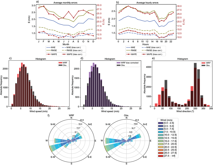
A comparison between WRF wind output and observations at La Rumorosa for the period 2015-2017 is provided in Figures 3 and S5. In general, WRF represents the annual cycle of the wind fairly well, particularly from August to October. During this time of the year the north of Baja California experiences high temperatures (with maximum above 40 ºC) and the smallest winds with a westerly component prevailing most of the time. On the contrary, the largest errors in the wind field are observed from January to April (Figs. 3a, b and S5a, b), when winds experience an increase in magnitude and the extreme temperatures decrease.
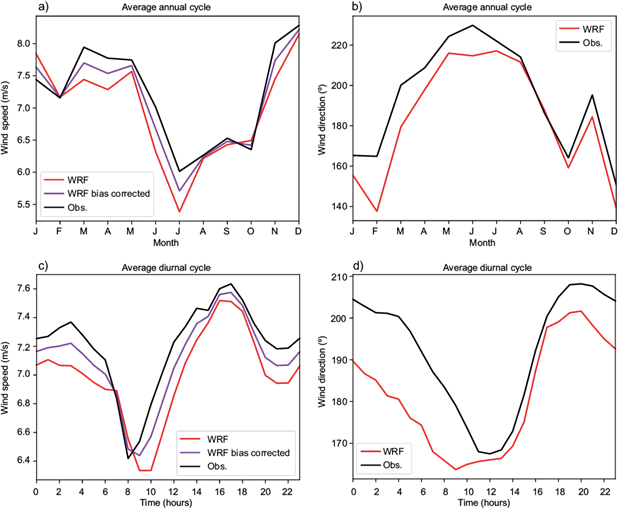
Fig. 3 (a, b) Average annual and (c, d) diurnal cycles of wind speed (left) and direction (right) in WRF simulations and in observations. Values are averaged for the period 2015-2017.
Figure 3c, d shows diurnal cycles of wind, demonstrating a good representation of the hourly averages of both wind speed and direction by the WRF model. The wind speed experiences a diurnal peak between 15:00 and 18:00 LT, which is also well reproduced by WRF. However, the hour of minimum wind speed in the diurnal cycle is not correctly predicted and represented later by WRF with respect to observations. Both annual and diurnal cycles of wind speed forecasts are closest to observations after the bias correction, with a MAE improved by around 1 m s-1 and a NMAPE by more than 10 percentage points.
Also shown in Figure S5 are the frequency distributions of modeled and observed winds and the wind rose plots. It is evident that the largest frequencies are adequately represented by WRF, particularly for wind speed (before and after bias correction), with the maximum frequencies between 5 and 7 m s−1. The histogram for wind direction shows a mismatch in the 0-50º directions, while the rest of the values are approximately well represented. For example, the two most frequent wind direction values coincide for both WRF and observations (around 245-275º). Finally, the wind rose plots show a good agreement between the two-time series of WRF and the observed wind; in particular, winds from the west and west-southwest directions prevail in both plots. Also, winds from the east-northeast are frequent in both plots; however, the winds from the northeast are more common in WRF than in observed data.
3.2 Estimation of wind power
This section evaluates the usefulness of the NWP model and the NN algorithm combined, for the site of interest in northwestern Mexico. Furthermore, the ability of this method is compared with wind power estimates obtained from two benchmark methods.
Table II indicates the average metrics computed over the evaluation period (the year 2017) for the two methods of wind power estimation. As shown, the NN exhibits slightly improved metrics with respect to DT and SVR. For instance, NMAPE decreases by six percentage points, and MAE and CRMSE by around 164 and 366 kW, respectively, with respect to DT estimates. In terms of mean bias and linear correlation, the performance is roughly similar between the three methods.
Table II Metrics of three methods for estimation of wind power*.
| Method | NMAPE (%) | MAE (kW) | CRMSE (kW) | Mean bias (kW) | Spearman ρ |
| NN | 6.97 | 187.53 | 371.58 | -23.22 | 0.98 |
| DT | 13.06 | 351.62 | 620.18 | -2.02 | 0.98 |
| SVR | 20.57 | 553.15 | 856.29 | -64.44 | 0.96 |
*Values represent an average of all samples for the year 2017. The average energy production in La Rumorosa wind farm for the period studied is 2692.30 kW.
NMAPE: normalized mean absolute percentage error; MAE: mean absolute error; CRMSE: centered root mean squared error; NN: neural networks; DT: decision trees; SVR: support vector regression.
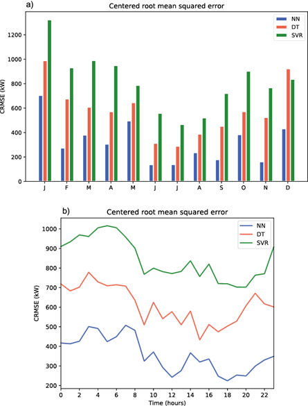
Monthly and hourly NMAPE are displayed in Figure 4. Similar plots, but for the CRMSE. are shown in Figure S6. In the annual cycle (Fig. 4a) lowest errors occur from June to August, coinciding with some of the months with lowest wind speeds (July and August in Fig. 3a) and smallest wind speed forecasting errors (Fig. S5a) in La Rumorosa. In those months, the errors of the NN and DT estimates differ little, while SVR exhibits the largest errors. Errors increase from December to April, when the NN performs notably better than the rest of the methods. Overall, NMAPE remained below 16% for the NN in the evaluation year, while errors reached up to 20 and 30% for the DT and SVR estimates, respectively. Figure 4b displays the mean hourly errors in two different seasons: May to October (MJJASO) and November to April (NDJFMA). As expected, errors are higher during the NDJFMA with respect to MJJASO season. Those errors decrease for the second part of the diurnal cycle in the NDJFMA season. The NN estimates exhibit similar errors during both seasons, while DT and SVR errors differ more between seasons.

Fig. 4 (a) Monthly and (b) hourly NMAPE for NN, DT, and SVR estimates for the year 2017. (NMAPE: normalized mean absolute percentage error; NN: neural networks; DT: decision trees; SVR: support vector regression.)
A comparison of the frequency distributions of wind power estimates from the three methods is shown in Figure 5. Overall, the three methods are able to adequately represent the probability distribution of real energy generation in La Rumorosa. NN overestimates wind power in the near zero range, while SVR underestimates it, indicating that these models tend to mismatch near-zero energy production. On the other hand, DT forecasts are correctly represented in the near-zero range. The SVR method tends to forecast more values in the extreme part of the distribution (> 10000 kW), which is erroneous. The rest of the energy generation values have roughly the same frequencies in the forecast and observations, for the three methods.
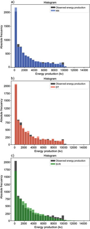
Fig. 5 Histograms of wind power forecasts for (a) NN, (b) DT, (c) SVR, for the year 2017. (NN: neural networks; DT: decision trees; SVR: support vector regression).
A further exploration of errors as a function of non-overlapping energy intervals is shown in Figure 6, which easily illustrates the energy ranges affected by the largest errors. This type of analysis can be relevant for wind energy markets since they can be interested in power generation above or below certain thresholds. Overall, MAE is smaller for NN than for the other methods at all the energy ranges. Errors for NN and DT peak between 5000 and 8000 kW, and decrease for the rest of the ranges, while for SVR errors maximize for large values, i.e., from 8000 to 10 000 kW, suggesting the method experiences difficulties in capturing larger energy peaks, overestimating them (Fig. 5c).
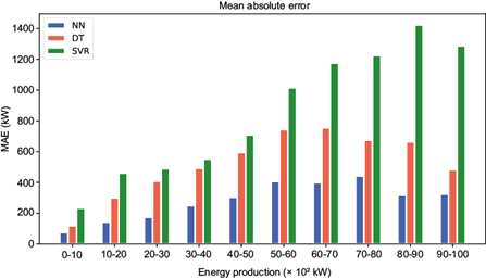
Fig. 6 Mean absolute error for 10 power generation ranges, from 0-1000 kW to 9000-10 000 kW, for NN, DT, and SVR estimates, for the year 2017. (NN: neural networks; DT: decision trees; SVR: support vector regression.
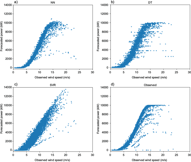
Power curves for the three power forecasting methods and the real power are shown in Figure 7, featuring the wind power against observed wind speed in La Rumorosa. As seen in the figure, the NN and DT power curves resemble the true curve, although with more dispersion in DT estimates. Wind speed above nominal velocities (14 m s-1) is more clearly represented in the DT model, and the NN has difficulties in accurately simulating the relationship between above-nominal wind speed and power. However, the forecasted power for the cut-in wind speed is more accurate in NN, which shows good agreement with the true curve. On the other hand, the SVR method does not reproduce well the observed power curve, evidencing a large mismatch between wind speed and power and a strong overestimation of wind power well above the maximum capacity of the plant.
4. Assessment of wind power forecast under special meteorological conditions
A previous work has reported that for some sites, wind speed and wind power forecast uncertainties depend on the weather situation (Lange and Waldl, 2001). Therefore, with the aim to further examine the wind power forecast performance in detail, its ability under special meteorological situations is evaluated in this section. To this end, we selected two events of frontal systems that arrived in Mexico by its north-western portion and transited over Baja California, thus affecting the La Rumorosa site. The first event corresponds to October 25-26 (hereinafter Oct25-26), and the second to November 6-9 (hereinafter Nov6-9), both in 2020. These cold fronts caused an increase in wind speed and a reduction of surface temperature that affected the dynamics of the boundary layer and, thus, the wind power forecast. Figure 8 shows the histogram of observed wind speed at La Rumorosa for 2015-2017, which compares the maximum wind speeds recorded at each event. Those values are above three standard deviations of the 7.24 m s−1 mean. The value that marks three standard deviations of the mean is also represented in Figure 8 and equals 18.04 m s−1. Therefore, the two cases are considered adequate for testing the behavior and ability of the NN model in forecasting wind power under synoptic features that cause an extreme turn of local meteorology, particularly wind speeds.

Fig. 8 Maximum wind speeds observed in two selected cases: October 25-27 (19.13 m s−1) and November 6-9 (22.5 m s−1).
Figures S7 and S8 show maps of surface temperature and wind fields for each case, evidencing the southwards advance of the cold air mass. In the Oct25-26 event, the cold front arrives in Baja California on October 26 during the morning hours and rapidly moves through the peninsula and northwestern Mexico, vanishing between the end of the day and the dawn of the next. On this day (October 26), Santa Ana winds affected several parts of southern California, USA (Nelson, 2020). This could explain the fact that winds behind the cold front have mostly a northerly component (Fig. S7). In the Nov6-9 case, the cold front arrives on November 7 during the early morning (between 00:00 and 03:00 LT) and moves southward at a slow pace. On November 8 at noon, the front becomes quasi-stationary over Baja California Sur, and a high-pressure system is present in the southwestern US. Then it dissipates by November 9.
To examine the ability of the wind power forecasts on these events, WRF simulations were carried out, and the NN, DT, and SVR models were applied to the outputs, following the same procedure as detailed in section 2.
4.1 October 25-27 cold front
Figure 9 shows the forecast and real hourly wind power for Oct25-27. The three methods fail to reproduce the real energy generation, particularly before the arrival of the cold front. After the arrival of the cold front, NN presents the largest errors (Fig. S9), forecasting values far above the observations, and this persists during most of the event. Instead, DT and SVR tend to be more accurate during the cold front.
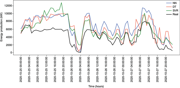
Fig. 9 Wind power on October 25-27: NN, DT, SVR, and real production. (NN: neural networks; DT: decision trees; SVR: support vector regression.)
Table III summarizes some relevant evaluation metrics as daily averages of hourly values. In general, the three wind power forecasting methods exhibit a bias in different parts of the time series from October 25 to 27, which are slightly larger for NN. Mean daily values of energy generation are overestimated by the three methods (positive bias in Table III). Daily NMAPEs are comparable for October 25, 2020, but are much smaller for the SVR method for October 26 and 27, ranging between 35 and 43%. Although errors for NN are large during the cold front, correlations still are high, as proven by values on October 26 and 27 (0.87 and 0.97, respectively).
Table III Daily average metrics during the Oct25-27 event: mean bias (kW), NMAPE (%), and Spearman ρ.
| Days | NN | DT | SVR | NN | DT | SVR | NN | DT | SVR |
| 2020-10-25 | 3023.14 | 2942.42 | 2961.62 | 52.28 | 51.12 | 53.03 | 0.21 | 0.29 | 0.43 |
| 2020-10-26 | 2284.52 | 1633.15 | 1280.11 | 66.32 | 51.02 | 43.93 | 0.87 | 0.64 | 0.62 |
| 2020-10-27 | 2449.20 | 1584.76 | 1006.91 | 67.08 | 51.22 | 35.53 | 0.97 | 0.75 | 0.92 |
NMAPE: normalized mean absolute percentage error; NN: neural networks; DT: decision trees; SVR: support vector regression.
4.2 November 6-9 cold front
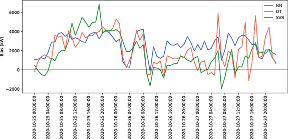
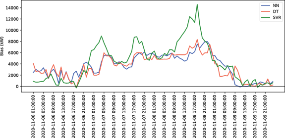
Figure 10 shows the time series of wind power for November 6-9, 2020. In this case, the highest errors are observed from November 7 at 00:00 LT (i.e., at the arrival of the cold front) until November 8 at 21:00 LT, when the cold front starts to dissipate. Biases are positive during all the event, ranging between 2000 and 6000 kW for the NN and DT models, while SVR exhibits the largest errors, with more than 10 000 kW in certain hours (Fig. S10). It is noticeable that before and after the passage of the cold front, all models produce significantly smaller errors. In general, the three wind power forecasting methods tend to overestimate the energy production during the two strong synoptic forcing events analyzed.
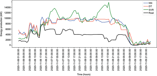
Fig. 10 Wind power on November 6-9: NWP-NN model, and real production. (NWP-NN: numerical weather prediction-neural networks).
Table IV shows daily averages of errors for the Nov6-9 case study. Before the cold front, mean daily biases ranged between 1000 and 2500 kW for the three forecasting methods, and afterwards they increased considerably. Furthermore, the biases of NN and DT models are comparable throughout the four days studied (see also Fig. S10). These methods evidenced a roughly similar behavior in forecasting wind energy under special meteorological conditions. The NMAPE is also similar for NN and DT during November 7 and 8, and the NN slightly improves afterward. The models also exhibit poor correlations during the same days, with a rapid increase on November 09, especially for NN.
Table IV Daily average metrics during the Nov6-9 event: mean bias (kW), NMAPE (%), and Spearman ρ.
| Days | NN | DT | SVR | NN | DT | SVR | NN | DT | SVR |
| 2020-11-06 | 2520.09 | 2261.08 | 1425.43 | 62.42 | 56.51 | 35.89 | 0.91 | 0.83 | 0.91 |
| 2020-11-07 | 4526.99 | 4415.35 | 6184.05 | 94.01 | 91.69 | 128.42 | -0.43 | -0.17 | 0.29 |
| 2020-11-08 | 5939.15 | 5886.52 | 8113.79 | 184.58 | 182.94 | 252.16 | 0.14 | 0.43 | -0.04 |
| 2020-11-09 | 1563.69 | 1328.14 | 1661.88 | 111.65 | 94.24 | 119.14 | 0.97 | 0.89 | 0.85 |
NMAPE: normalized mean absolute percentage error; NN: neural networks; DT: decision trees; SVR: support vector regression.
5. Discussion and conclusions
This paper proposes a hybrid method for day-ahead forecasts of wind energy and tests its functionality and performance for a wind farm in northwestern Mexico, by comparing it with two widely used benchmark approaches. The method uses an NWP model to forecast meteorological variables, which are the input of a non-supervised NN algorithm. A clear advantage of this approach is the ability to post-process NWP model outputs, accounting for low model resolution and uncertainties of physical models, and correcting the resulting biases (Novak et al., 2014). Another beneficial characteristic of this method is the capability to incorporate physical aspects of local weather conditions in the site of interest into the wind power estimates. Finally, the ability to capture non-linear relationships between meteorology and power generation by the NN is also a good feature of this methodology. On the other hand, some of the drawbacks of this method are the requirement of a historical dataset to train the artificial intelligence model, the need to develop a single model for a specific site, and the need for computer resources to run the NWP model.
We have used DT and SVR algorithms as benchmark models to compare the proposed methodology against them. Results show that the NN is capable of surpassing the performance of both DT and SVR, although the former shows skills comparable to the NN for hourly errors during the MJJASO season. The SVR method showed poorer skills for wind power forecasting, and exhibited large errors above the plant maximum generation capacity. In general, hourly bias tend to be smaller for the NN model as shown in Figure S11; they are mostly concentrated around zero while DT tends to exhibit more dispersion from zero and SVR has a slight negative bias in high wind power values. The improvement in performance of the NN is evident by a reduction in monthly errors by 6 and 13 percentage points with respect to DT and SVR, respectively (Table II). Thus, the proposed NN model can supply wind power forecasts that better represent the overall relationship between observed meteorological variables and wind energy than the two AI methods.
An objective comparison of our results with previous approaches would be insightful; however, it is limited because results depend on metrics definition, evaluation period, and plant maximum capacity, among other factors. Nevertheless, a qualitative assessment allowed us to confirm the usefulness of our results in the context of previous works. The NN forecasts exhibited monthly errors ranging between 3 and 15%, and hourly errors between 5 and 9% (Fig. 4), thus representing a good performance with respect to the average model’s performance in the medium term (6-24 h ahead predictions), which range between 10 and 20% (Okumus and Dinler, 2016). For example, Alessandrini et al. (2015) used an analog ensemble method for wind power forecasting over complex topography and obtained a MAE (normalized by plant nominal power) of around 10% for a 18-24 h ahead forecast horizon, while our monthly MAEs (normalized by plant average power production) are below 9% (except for January). The same applies to our hourly MAEs (between 5 and 9%). More recently, Duarte et al. (2021) reported a monthly percentage MAE of 12.6% for wind power estimates using NWP, while our monthly NMAPE (averaged from January to December) is 6.93%.
The present work also assessed the behavior of the wind power forecasting system under special meteorological conditions in La Rumorosa, such as cold fronts. It was seen that model’s ability declines, which was consistent among all the methods compared. One of the main sources of these large errors under cold front conditions is possibly originated in insufficient training data, since extreme meteorological conditions occur at a low frequency, with a scarce representation in the training dataset, which can limit the model’s learning process. Therefore, the AI and NN models fail to capture the complex dynamics of extreme events. Other approaches, like hierarchical algorithms (Peláez-Rodríguez et al., 2022), must be applied to improve the prediction skills of NN models on extreme events while preserving the prediction performance for regular conditions.
In conclusion, the method presented and evaluated in this paper is a valid tool for wind power forecasting with high accuracy under typical conditions. This method can be operational and provide decision support to grid operators, facilitating the implementation of renewable energy resources and gaining confidence in them.
Further work needs to be done to increase the accuracy of NWP models, due both to horizontal resolution and physical uncertainties, since they play an important role in hybrid methods of wind power forecasting. Besides, there is still much to do regarding the design of NN algorithms that can accurately forecast renewable power during extreme meteorological episodes, which is still problematic for artificial intelligence algorithms.