


 nueva página del texto (beta)
 Inglés (pdf)
 Artículo en XML
 Referencias del artículo
 Enviar artículo por email
 Citado por SciELO
  Similares en
SciELO
Similares en
SciELO 
 Permalink
1. Introduction
Extreme events caused by deviations from the precipitation norm, such as floods and droughts, directly affect human activity, producing impacts not only on the economy but also on the environment and society in general (Montealegre, 2009). Deviations from the precipitation norm are due to climate variability and can arise from multiple causes varying from regional atmospheric circulation anomalies to global climatic oscillations associated with ocean-atmosphere interactions (Kousky et al., 1984). Moreover, climate variability has been enhanced by climate change, principally over the late 20th and early 21st centuries.
To diminish the impacts of extreme meteorological events, high-quality and reliable precipitation forecast tools are essential in the development of mitigation strategies (Anshuka et al., 2019). In fact, forecasting climatic variables through the study of teleconnections has become increasingly common and valuable for different planning activities (Bravo et al., 2006).
Teleconnections are significant correlations between simultaneous or lead/lag fluctuations in meteorological phenomena from separate geographical areas (Wallace and Gutzler, 1981; Misra, 2020), e.g., the link between sea surface temperature (SST) in the tropical Pacific and seasonal rainfall in Mexico. In this study, correlations between monthly precipitation and the three main modes of climate variability that have affected precipitation regimes over Mexico during the late Holocene are analyzed (Metcalfe et al., 2015; Park et al., 2017). These modes are based on SST patterns of the Atlantic and Pacific oceans and are identified as the Pacific Decadal Oscillation (PDO), El Niño Southern Oscillation (ENSO) and the Atlantic Multidecadal Oscillation (AMO). To our knowledge, this is the first work that analyzes the influence of AMO, ENSO, and PDO on meteorological patterns in northern Mexico under a climate classification approach.
Firstly, AMO is a marked signal of the multidecadal variability observed in North Atlantic SSTs. Although it was first named by Kerr (2000) and was later defined as an index by Enfield et al. (2001), this pattern has been identified by scientists since the 1960s and paleoclimate proxies suggest it has been occurring for at least a thousand years. Enfield et al. (2001) defined the AMO index as the ten-year running mean of Atlantic SST anomalies north of the equator; the cool and warm phases follow medium-term cycles of 20 to 40 years (Jiménez, 2015) and have peak-to-peak variations of around 0.4 ºC (Enfield et al., 2001). This oscillation is known to affect climatic variables like air temperature and rainfall over the Northern Hemisphere (NOAA AOML, 2005). Particularly, warm phases of AMO (AMO+) have been associated with an increased frequency and/or severity of droughts in North America and hurricanes in the Atlantic (NOAA AOML, 2005; Curtis, 2008).
Similarly, interdecadal changes in the North Pacific SST have been reported since the past century. Pacific fishermen were the first to notice this pattern due to differences in salmon catch; later on, this pattern was named as PDO by Mantua et al. (1997). PDO encompasses the monthly variations of Pacific SST poleward of 20º N and follows a periodicity of 15 to 20 years (Jiménez, 2015). When PDO is in a warm phase (PDO+), the central North Pacific tends to be cooler than normal and SST along the west coast of the Americas tends to be warmer; the opposite occurs during a cool phase of PDO (PDO-) (Mantua and Hare, 2002). Furthermore, climatic effects of this oscillation can be responsible for up to 50% of the annual precipitation variability over the southwestern region of North America (Méndez et al., 2010). In particular, studies have reported a link between wet (dry) periods over northern Mexico and PDO+ (PDO-) (Woolhiser, 2008; Méndez et al., 2010; Gutiérrez-García et al., 2020;).
Lastly, ENSO takes place in the central and eastern equatorial Pacific. The first written record of the El Niño phenomenon was published in the Bulletin of the Geographical Society of Lima in 1892 (Carrillo, 1892), yet observations of its weather impacts date back to 1525 (Hanley et al., 2003). To identify this phenomenon, one of the most commonly used indices in the study of teleconnections, and NOAA’s standard, is the Oceanic El Niño Index (ONI), which measures SST anomalies of +/-0.5 ºC in an equatorial Pacific region called El Niño 3.4 (5º N-5º S, 170º-120º W) quarterly (Glantz and Ramírez, 2020). El Niño ocean current couples with the Southern Oscillation atmospheric current and feedback processes allow the phenomenon to fluctuate between its negative phase (La Niña) and positive phase (El Niño). ENSO is the large-scale ocean-atmospheric mode that has the greatest effects on interannual climate variability around the world (Díaz-Esteban and Raga, 2018; Durán-Quesada et al., 2020) and in Mexico (Trenberth, 1997; Díaz et al., 2002; Cerano-Paredes et al., 2013). Notably, studies show that in northern Mexico, El Niño (La Niña) events correspond to humid (dry) periods during both summer and winter seasons (Seager et al., 2009; Stahle et al., 2012; Campos et al., 2020).
The potential of studying those climate oscillations lies in providing insight into how fluctuations in precipitation may be coupled with different time scale stimuli; thus, contributing to the development of long-, medium- and short-term programs designed to mitigate the impacts of extreme events. Extreme hydrometeorological events represent a major threat not only for civilizations and socioeconomical conditions, but also for environmental features such as ecosystems, agriculture, and hydrology. More importantly, since northern Mexico is a drought prone region, given its arid climate and erratic rainfall, the occurrence of one meteorological drought could cause multiple effects that can persist even after the extreme event has concluded (Campos et al., 2020).
In fact, water scarcity has had a long history of repercussions in the country, going from the fall of various ancient civilizations to the social unrest that led to the Mexican Revolution and Independence, as well as the current social conflicts being faced at present due to water shortages in the North. Furthermore, the vulnerability of northern Mexico to these types of natural hazards is expected to increment given the significant trends in temperature increase and reduction of precipitation that some authors estimate for the region (Cavazos et al., 2020).
The observed and expected impacts enhance the representativeness of the region for the study and increase the applicability of the results. At the same time, the state of Tamaulipas as well as the Baja California peninsula were selected as both regions encompass the eastern and western sides of northern Mexico and have different climate conditions. Two regions with different physical characteristics were studied to evaluate if the existent atmospheric and terrestrial conditions exerted any effect on the comparative analysis of linear correlations.
By applying Pearson and Spearman correlation analyses, this work aims to identify phases of AMO, ENSO, and PDO that can be related to periods of above/below normal precipitation over dry and semi-dry regions of the Baja California peninsula and Tamaulipas. A second research objective is to identify the similarities and differences in the results obtained from the correlation analyses. Lastly, findings in this study will be useful for local authorities, considering that the information generated contributes to the development of meteorological forecasts applicable to different productive activities, which in turn intend to mitigate and reduce the effects of droughts and floods.
2. Materials and methods
2.1 Study area
The Baja California peninsula, comprised by the states of Baja California and Baja California Sur, is characterized by a very dry climate, also called dry desert climate with extreme temperatures and scarce rains. The minimum-maximum temperatures can range from 5 to 35 ºC and average yearly precipitation from 100 to 300 mm (García, 1964; Vidal, 2005). The low values of relative air humidity, around 40% during May, are driven by dry wind subsidence and the effects of cold sea currents that impede evaporation processes (Vidal, 2005). On the other hand, nearly half of the state of Tamaulipas has a dry and semi-dry climate, also called dry steppe climate, with average annual temperature values above 18 ºC and 300 to 600 mm of average rainfall per year (Vidal, 2005). The low precipitation values are partly a consequence of the anti-trade wind subsidence, which carries little humidity (Vidal, 2005).
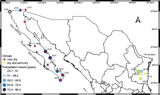
Sixteen climate stations managed by the Servicio Meteorológico Nacional (Mexican National Meteorological Service, SMN) were selected upon three criteria. Firstly, the effective length of the precipitation record had to be greater than 25 years. Secondly, the Standardized Precipitation Index (SPI) data set from the station needed to be available in the Comisión Nacional del Agua (National Water Commission, Conagua) public record. Thirdly, the site had to belong to a region with either very dry, or dry and semi-dry climate category, according to the modifications to the Köppen climate classification system proposed by García (1964), who adjusted the categories to the particular physical conditions in Mexico. The climate stations selected to conduct this study are shown in Figure 1.
2.2. Precipitation data
Regarding precipitation data, the SPI was chosen for the analysis since it is one of the most widely used indices among researchers given its simplicity, its adaptation to different time scales, and its dependence on a single parameter, which is precipitation (WMO, 2012). Furthermore, experts who participated in a World Meteorological Organization workshop on drought concluded that, as a general recommendation, national meteorological and hydrological services around the world should use the SPI to characterize meteorological drought (Hayes et al., 2011). Given the above mentioned, the three-month period SPI (SPI-03) was chosen as it depicts short and medium term moisture conditions that can describe seasonal estimations of precipitation (WMO, 2012). Monthly SPI-03 data for the selected climate stations were obtained from the drought monitor tool generated by Conagua (2022), available for the general period of 1951-2021.
The general period of study comprises a total of 71 years from January 1951 to December 2021, which is a sum of 852 monthly values per station. Nevertheless, there are some stations with shorter records that are reflected in the fourth column of Table I. The discontinuity in the records of climate stations is quite common. Interruptions appear due to multiple factors, including the lack of proper funding. Table I shows the percentage of missing data in the SPI-03 monthly records for each climate station.
Table I Percentage of monthly missing SPI-03 data for each station.
| State | Station | Name | Total monthly data | Monthly data without record | Percentage of missing data |
| Baja California | 2033 | Mexicali (DGE) | 852 | 22 | 2.58% |
| 2037 | Presa Morelos | 732 | 106 | 14.48% | |
| 2038 | Presa Rodríguez | 852 | 8 | 0.94% | |
| 2046 | San Felipe | 852 | 113 | 13.26% | |
| Baja California Sur | 3005 | Cabo San Lucas | 852 | 86 | 10.09% |
| 3030 | La Ribera | 852 | 28 | 3.29% | |
| 3035 | Loreto (DGE) | 852 | 47 | 5.52% | |
| 3038 | Mulegé | 816 | 78 | 9.56% | |
| 3068 | Villa Constitución | 780 | 49 | 6.28% | |
| 3073 | Gustavo Díaz Ordaz | 612 | 28 | 4.58% | |
| 3074 | La Paz (DGE) | 852 | 37 | 4.34% | |
| Tamaulipas | 28028 | El Barretal I | 852 | 139 | 16.31% |
| 28070 | Padilla | 852 | 35 | 4.11% | |
| 28074 | Paso de Molina | 720 | 18 | 2.50% | |
| 28087 | San Gabriel | 732 | 8 | 1.09% | |
| 28152 | Soto La Marina | 576 | 110 | 19.10% | |
| Average percentage of missing data | 7.38% | ||||
DGE: Dirección General del Estado. It refers to stations enabled around 1950-1960 by the former Ministry of Agriculture and Water Resources.
Since the average percentage of missing values in all stations is smaller than 8%, no method was used to estimate the missing values. Rather, by applying a piece-wise approach, the values without data were not considered in the computation of correlations. Data from climate stations with a percentage of untaken readings greater than 5 and 10% were used. Although this might affect the accuracy of the results, it is a common practice in national studies given the lack of precipitation data in the country (Caso et al., 2007; Peralta-Hernández et al., 2008; Hidalgo et al., 2019).
The stations considered for the precipitation data meet the following characteristics: no more than 20% of information is missing from each historical record, the series have at least 25 years of effective records, and all climate stations report information in an operational manner. In addition, an analysis of the variance homogeneity was performed by means of the nonparametric Levene test (Levene, 1961). Using the median as the measure of centrality, this statistical test was applied to groups of stations within a maximum radius of 124 km. All the p-values indicated that there is no significant difference between the dataset variances at a 95% confidence interval.
For the 228 variables studied (monthly registers of 16 climate stations and three climatic indices) the average number of observations is 71.75 and all individual variables have at least 35 observations.
2.3. Climatic data
Data for the three climate indices under study were obtained from the following sources: firstly, for the monthly AMO index record, the information was obtained from NCAR (2022); secondly, for the ONI index, the data was obtained from the Climate Prediction Center (CPC, 2022); lastly, for the PDO index, the data series was obtained from the National Centers for Environmental Information (NCEI, 2022).
2.4 Methods
The multifactorial origin of droughts has considerably hindered the construction of a universal method for their forecast (Martínez-Austria and Díaz-Jiménez, 2018). For this reason, the research was limited to the study of the statistical relationships that a single drought index has shown with respect to three climatic indices that seem to be the most important for the study region.
Through a systematic review of background studies using the PRISMA approach (Page et al., 2021), several methodologies applicable to the analysis of teleconnections were identified. Correlations were recognized within the most commonly used methods, in which Pearson (González-Elizondo et al., 2005; Potter et al., 2008a, b; Llanes-Cárdenas et al., 2018; Campos et al., 2020) and Spearman correlations (Méndez et al., 2010; Návar, 2015; Díaz-Esteban and Raga, 2018; De Luca et al., 2020) showed satisfactory results for Mexico. Both analyses were applied to monthly records of SPI-03 paired with monthly data of AMO, ONI, and PDO for the period 1951-2021. The data sets were first evaluated for linearity using graphical methods and then assessed for normality using both empirical and hypothesis test methods. The statistical significance of the correlation values was established for α = 0.05 or a 95% confidence interval, using a hypothesis test method.
2.5 Pearson and Spearman main differences
Pearson (1896) defined a correlation coefficient that well described the strength of the linear relationship between two quantitative variables. Years later, Spearman (1904) modified Pearson’s coefficient and created a new method that was suitable for two variables which cannot be measured quantitatively. The sample Pearson correlation coefficient (Eq. 1) is computed analogously to the sample Spearman correlation coefficient (Eq. 2); however, in the Spearman method x and y are first transformed into ranks between 1 and N. In the case of two identical data values (tied observations), they obtain the same average rank.
In general, the purpose of each coefficient is different. While r measures the level of linearity between two variables, ρ is more suitable when estimating their monotone association (de Winter et al., 2016). Spearman’s rank correlation coefficient is nonparametric, and several authors suggest it is more robust to heavy-tailed distributions and less sensible to outliers than the Pearson correlation coefficient. Instead, Pearson’s coefficient is more appropriate for light-tailed distributions, and it is parametric, meaning that it generally requires the two variables to be normally distributed, although some authors have found it is applicable when a moderate deviation from the normal distribution exists. Spearman’s coefficient has been less frequently used than Pearson’s coefficient, nevertheless, the former is helpful when the distribution of data makes the latter undesirable or misleading (Hauke and Kossowski, 2011).
3. Results and discussion
3.1 Variable characteristics
In order to understand the type of relationship between the different variables under study, scatter plots were created for monthly records of SPI-03 of two randomly selected climate stations in each state (Baja California, Baja California Sur, and Tamaulipas) paired with AMO, ONI, and PDO monthly series. Figure 2 illustrates certain examples where linear relationships were found to be statistically significant (p-value < 0.05).
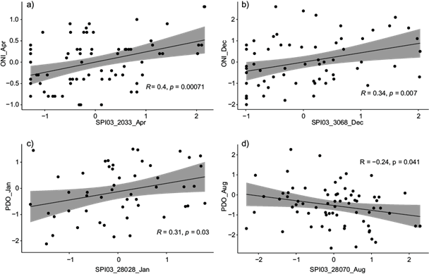
Fig. 2 Evaluation of the linear relationship between SPI-03 and (a) ONI in Baja California, for April monthly series; (b) ONI in Baja California Sur, for December monthly series; (c) PDO in Tamaulipas, for January monthly series, and (d) PDO in Tamaulipas, for August monthly series.
Linearity assessment, in terms of statistical significance showed that the relationship between precipitation and the three climate indices can be assumed to be linear. The magnitude of R in Figure 2a-d falls within previously reported ranges for northern Mexico (Díaz et al., 2002; Llanes-Cárdenas et al., 2018). Slightly stronger correlation coefficients were obtained for SPI-03 associations with ONI, followed by associations with PDO and AMO. This is consistent with previous findings which consider ENSO as the most relevant factor of the interannual climatic variation in Mexico (Stahle and Cleaveland, 1993; Trenberth, 1997; Díaz et al., 2002; Cerano-Paredes et al., 2013).
After checking linearity, normality was evaluated in order to understand the behavior of the data, which will in turn define the suitability of the correlation method. For this purpose, both empirical and hypothesis test methods were applied to randomly selected monthly registers of AMO, ONI, PDO, and SPI-03. The registers were chosen at random using the Mersenne Twister algorithm to ensure unbiased selection.
Column 2 in Table II shows the results of the Shapiro-Wilk test, which proves normality when p-value > 0.05. Alternatively, columns 3-5 reveal the empirical rule evaluation, also referred to as the three-sigma rule, which indicates normality conditions when at least 68% of the observations fall within the first limit µ ± σ, 95% within the second limit µ ± 2σ, and 99.7% within the third limit µ ± 3σ. In this way, the criteria were applied to registers of the climatic indices and registers of SPI-03 from two stations in each state (Baja California, Baja California Sur, and Tamaulipas), excluding the stations already evaluated for linearity. Likewise, registers from temporarily separate months were considered to contemplate climatic variability within a year.
Table II Normality tests for precipitation and climatic oscillations monthly data sets.
| Hypothesis tests p-values | Percentage of data within empirical rule limits | |||
| Monthly data sets | Shapiro-Wilk | µ ± σ | µ ± 2σ | µ ± 3σ |
| SPI03_2037_Feb | 0.1242 | 60.42% | 100.00% | 100.00% |
| SPI03_2046_Sept | 0.0000 | 87.50% | 93.75% | 98.44% |
| SPI03_3005_Oct | 0.7020 | 68.25% | 93.65% | 100.00% |
| SPI03_3073_Jan | 0.2073 | 68.09% | 97.87% | 97.87% |
| SPI03_28087_Dec | 0.4147 | 70.00% | 98.33% | 100.00% |
| SPI03_28152_May | 0.2300 | 72.97% | 91.89% | 100.00% |
| AMO_Aug | 0.0005 | 57.53% | 100.00% | 100.00% |
| AMO_Apr | 0.0004 | 60.27% | 100.00% | 100.00% |
| ONI_Mar | 0.1303 | 72.22% | 94.44% | 100.00% |
| ONI_Nov | 0.1834 | 69.44% | 95.83% | 100.00% |
| PDO_Feb | 0.2904 | 63.69% | 98.21% | 99.40% |
| PDO_Oct | 0.6625 | 63.69% | 97.02% | 100.00% |
Bold numbers indicate non-normality.
As Table II shows, under certain criteria applied, some variables do not follow the precise behavior of a normal distribution. What is interesting about the data in this table is that the empirical rule resulted in more non-normal outcomes than the hypothesis test. Concerning the hypothesis test, variables SPI03_2046_Sept, AMO_Aug and AMO_Apr exhibited p-values below the 0.05 threshold in each of the three normality tests. Figure 3 shows the quantile-quantile plots for these variables. Under the empirical rule criteria, a larger number of variables revealed non-normal characteristics as depicted in Table II. Nevertheless, these results are markedly influenced by the presence of outliers as shown in Figure 4 for variables SPI03_3073_Jan and PDO_Feb shown in Figure 4.
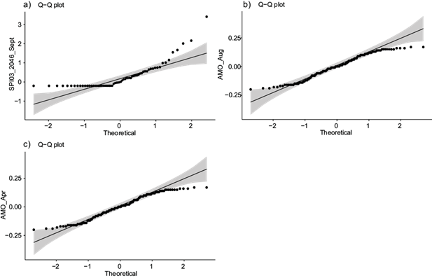
Fig. 3 Quantile-quantile plots of variables. (a) SPI03_2046_September, (b) AMO_August, and (c) AMO_April, whose hypothesis test results indicate a non-normal behavior.
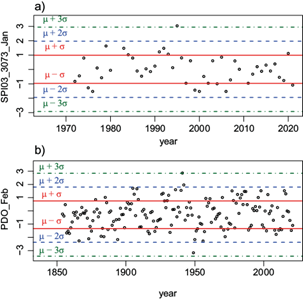
Fig. 4 Empirical rule limits for variables that encompass outliers: (a) SPI03_3073_Jan, and (b) PDO_Febr.
Moreover, this is one of the few studies in the field that develops a variable normality assessment. Remarkably, through the systematic review of previous studies where 75 documents were examined using the PRISMA methodology, only two authors reported normality evaluation in the use of correlation analysis (Návar, 2015; Llanes-Cárdenas et al., 2020). Statistical errors such as not considering the variable characteristics before applying correlation analysis are frequent; in fact, Ghasemi and Zahediasl (2012) affirm that about 50% of the published scientific articles have at least one statistical error. In this way, the variable normality assessment adds advantageous value to the present work and helps evaluate the validity of the results.
Given the absence of normal characteristics revealed by some variables as shown in Table II, selecting Spearman correlations would be a cautious decision. However, numerous authors assure Pearson’s robustness in the absence of normality. Specially, Ghasemi and Zahediasl (2012) state that when the sample size is greater than 30 or 40 observations, the violation of the normality assumption loses importance. Hence, given that all individual variables have at least 35 observations, both Pearson and Spearman correlations were applied, as detailed in section 3.2.
3.2 Pearson and Spearman correlations
Both Pearson and Spearman correlation analyses were applied to each 12 monthly SPI-03 registers, paired with the 12 monthly registers of AMO, ONI, and PDO for the period 1951-2021. In this way, six correlation matrices were computed for each of the 16 climate stations under study. The results of both correlation analyses exhibited similar behavior, suggesting that Pearson and Spearman correlation coefficients behave similarly when describing teleconnections in the study area.
The correlation matrices presented in Figures 5, 6 and 7 summarize the results of all 16 climate stations, clustering them into states and comparing Pearson vs. Spearman outcomes. Figure 5 condenses the correlations for stations 2033, 2037, 2038, and 2046, located in Baja California; Figure 6 compiles results of stations 3005, 3030, 3035, 3038, 3068, 3073, and 3074, located in Baja California Sur; and Figure 7 gathers correlations in stations 28028, 28070, 28074, 28087, and 28152, located in Tamaulipas. A layering method using transparencies was applied to depict multiple stations in a single figure.
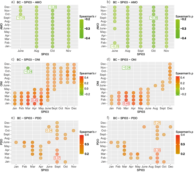
Fig. 5 Pearson and Spearman correlations between SPI-03 indices recorded in Baja California (BC) and (a, b) AMO, (c, d) ONI, and (e, f) PDO for the period 1951-2021. Only statistically significant results are shown (p < 0.05) and the numbers inside squares indicate the maximum and minimum values of the correlation coefficients.
As can be compared from Figure 5a, b, the results of Spearman correlation analysis exhibited better performance when correlating SPI-03 and AMO in Baja California in terms of the amount of statistically significant correlations (p < 0.05), whereas the opposite occurs for SPI-03 and ONI correlations (Fig. 5c , d) where Pearson’s analysis accomplished more significant correlations. For the PDO teleconnections (Fig. 5e, f), both correlation analyses produced similar results as to total number of statistically significant correlations, with an overall difference of less than 10%. On the other hand, it is apparent from Figure 5 that the general magnitude of the correlations does not vary substantially depending on the type of correlation analysis, except for a slight difference in SPI-03 teleconnections with PDO and AMO, where a greater correlation value was displayed by Pearson’s r for the former and by Spearman’s ρ for the latter.
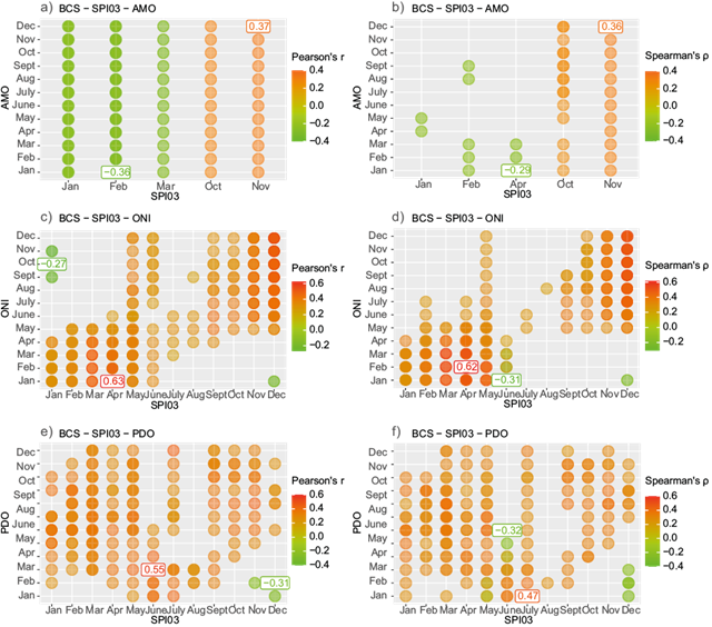
Turning now to Figure 6, Pearson’s correlations revealed a moderately greater potential when estimating the total amount of statistically significant results in Baja California Sur regarding SPI-03 teleconnections with AMO (Fig. 6a, b) and ONI (Fig. 6c, d), whereas in teleconnections with PDO (Fig. 6e and 6f), the difference in the number of statistically significant results obtained by Spearman’s and Pearson’s correlation analyses was < 1%. Additionally, a comparison of the maximum and minimum correlation values reveals that Pearson’s r reached greater magnitudes for AMO teleconnections, in both minimum and maximum values, as well as in maximum values for ONI and PDO teleconnections, while Spearman’s ρ arrived at greater minimum values for both ONI and PDO teleconnections.
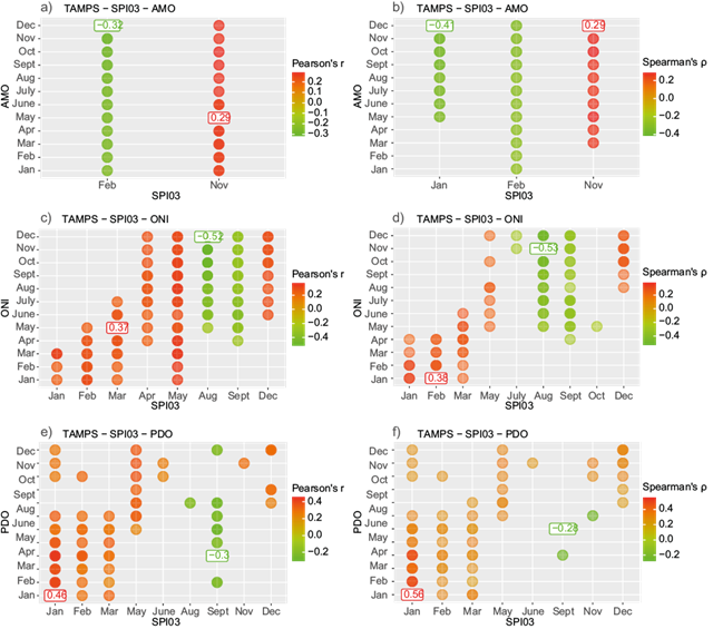
Like the Baja California results, Figure 7 illustrates that for the state of Tamaulipas, Spearman’s correlations surpass Pearson’s in terms of the amount of statistically significant correlations, regarding the SPI-03 and AMO associations (Fig. 7a, b), while the opposite occurs for SPI-03 and ONI correlations, where more significant correlations are achieved with Pearson’s analysis (Fig. 7c, d). For the PDO teleconnections (Fig. 7e, f), both correlation analyses showed similar behavior with respect to statistically significant correlations with a total difference of less than 10%, as observed for Baja California. When comparing the magnitude of the results presented in Figure 7, it can be seen that Spearman’s ρ exhibited greater absolute values for both positive and negative SPI-03 correlations with AMO and ONI. Alternatively, for the SPI-03 teleconnections with PDO, Pearson’s r produced a lower minimum correlation value and Spearman’s ρ presented a higher maximum correlation value.
An overall analysis of Figures 5-7 indicates that ONI and PDO have the greatest impact in the SPI-03 observed for Baja California, Baja California Sur, and Tamaulipas. These results are consistent with those reported by Fuentes-Franco et al. (2018), who found that the interannual precipitation variability over northern Mexico, and specially over Baja California, is strongly linked to ENSO and PDO. In addition, the response of SPI-03 to these two modes of climate variability demonstrated similar behavior, in terms of positive/negative signs throughout the year. This is also in accordance with analyzes that show that the PDO effect patterns are similar to those of ENSO and that these two modes might even depend on each other (Méndez et al., 2010; De Luca et al., 2020; Durán-Quesada et al., 2020; Gutiérrez-García et al., 2020).
Turning now to the direction of the results, Figures 5 and 6 show that both PDO and ONI have mostly positive correlations with SPI-03 throughout the year in the Baja California peninsula (Baja California and Baja California Sur), supporting the findings of previous studies (Magaña et al., 2003; Reyes-Coca and Troncoso-Gaytán, 2004; Méndez et al., 2010; Méndez and Magaña, 2010; Stahle et al., 2020). The ONI correlations reach a maximum in early spring (March-April) with the highest values being r max = ρ max = 0.45 for Baja California, and r max = 0.63 for Baja California Sur, while the maximum values of PDO correlations are observed during summer-autumn with coefficients of r max = 0.37 for Baja California (September) and r max = 0.55 in Baja California Sur (June), all coefficients significant at the 0.05 level.
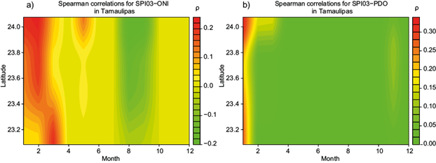
Figure 7 illustrates ONI and PDO influences over the state of Tamaulipas, where a positive correlation with SPI-03 prevails during most of the year with maximum values during the winter months of ρ max = 0.38 for ONI (February), and ρ max = 0.56 for PDO (January) (p < 0 .05). At the same time, negative SPI-03 correlations with ONI and PDO appear for Tamaulipas in the late summer and early autumn months as stated by Quiroz-Jiménez et al. (2018) for central-northern Mexico, and by Roy et al. (2020) for northeast Mexico, with minimum values of ρ min = -0.53 for ONI (August), and r min = -0.53 for PDO (September), all coefficients significant at the 0.05 level.
Conversely to the behavior of ONI and PDO teleconnections, AMO shows a similar pattern in Baja California Sur and Tamaulipas (see Figs. 6 and 7), where a negative correlation appears in the first months of the year (January-April), reaching minimum values of r min = -0.36 (Baja California Sur) and ρ min = -0.41 (Tamaulipas), and a positive correlation by the end of the year (October-November) with maximum coefficients of r max = -0.37 (Baja California Sur) and r max = ρ max = 0.29 (Tamaulipas), supporting findings of previous works (Méndez and Magaña, 2010; Durán-Quesada et al., 2020). Moreover, Baja California presents a rather different pattern in AMO teleconnections. Here negative correlations appear throughout all seasons of the year in accordance with previous studies (Méndez and Magaña, 2010; Cavazos et al., 2020; Stahle et al., 2020), reaching minimum correlation coefficients of ρ min = -0.38 (October).
3.3 Correlations without lag
Since ONI and PDO have the greatest effect on precipitation over the three states, Figures 8 and 9 show the behavior of these teleconnections along the spatial extent of the Baja California peninsula and Tamaulipas. Spearman SPI-03 correlations with ONI and PDO are shown in Figures 8 and 9 for monthly series without lag (January-January, February-February…, December-December) as no assumptions are violated for that method. It is shown that zero-lag positive correlations appear during the period January-May for ONI and PDO in both regions, except for Tamaulipas where the PDO correlation emerges stronger in January and disappears around March. Months later, negative zero-lag correlations occur throughout July-October for ONI in Tamaulipas. Furthermore, by the end of the year, positive zero-lag correlations come into sight once more during the months of August-December for PDO and ONI teleconnections in the Baja California peninsula.
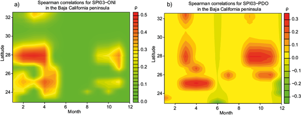
Fig. 8 Zero-lag correlations between SPI-03 indices recorded in the Baja California peninsula and (a) ONI and (b) PDO for the period 1951-2021. Only statistically significant results are shown (p < 0.05).
3.4 Mechanisms involved in teleconnection patterns
As discussed, ONI and PDO have equivalent effects over Baja California and Baja California Sur and a slightly different response over Tamaulipas, where an opposite correlation occurs during the late summer and early autumn months. During these months, the hurricane season mainly impacts the hydroclimatic variability in northeastern Mexico, hence, storms of these type interfere with the signal of teleconnections. At the same time, the presence of mountainous regions such as the Sierra Madre Oriental exert an important control over precipitation in Tamaulipas as they interact with wind patterns that transport moisture from the Gulf of Mexico.
On the other hand, numerous authors associate the wet conditions over the Baja California peninsula during El Niño years to the increment of winter storm tracks caused by the strengthening and southward shift of the subtropical jet stream (Durán-Quesada et al., 2020; Gutiérrez-García et al., 2020). In turn, the strengthening of the subtropical jets in both hemispheres during El Niño years is created by the intensification of the Hadley Circulation generated by the more uniformly warm SST in the equatorial Pacific, which reduces the east-west temperature gradient (Kousky et al., 1984). Thus, the latitudinal position of subsidence from the Hadley Cell is affected by both ENSO and PDO (Méndez and Magaña, 2010).
Likewise, the anomalous warmer waters extending to the west coasts of California and Mexico during El Niño enhance precipitation through the increase of precipitable water vapor in storm air masses (Minnich et al., 2000). Nicholas and Battisti (2008) state that the El Niño phases tend to intensify the North Pacific storm track which extends farther eastward and produces wet conditions over northwestern Mexico. In addition, Magaña et al. (2003) link the increase in the number of mid-latitude frontal systems traveling across northern Mexico during positive ENSO phases to the Pacific North American (PNA) pattern, a quasi-stationary Rossby wave generated by the anomalous convective heating over the eastern and central Pacific.
Alternatively, the similar SPI-03 response to AMO in Baja California Sur and Tamaulipas might be attributable to the latitudinal position of both states (22º-28º N), which in turn dominates numerous atmospheric processes, such as moisture transport, convective activity, wind patterns, and pressure gradients. On the other hand, Baja California is located northward of Baja California Sur and Tamaulipas (28º-32º N), situated on the equatorward margin of the planetary jet stream where the Mediterranean climate (characterized by winter precipitation and summer drought) of higher latitudes changes into more desertic climates in lower latitudes (Minnich et al., 2000). This explains to some extent the distinct teleconnection pattern of AMO over Baja California when compared to that of Tamaulipas.
As stated by Ruprich-Robert et al. (2018), positive phases of Atlantic multidecadal variability are related with warmer tropical SST, which generates a Matsuno-Gill response that produces downward motion in the upper troposphere over northern Mexico; hence, the upper to mid-troposphere warms and the atmospheric relative humidity decreases, as does the cloud cover. Similarly, Cavazos et al. (2020) suggest that the positive phases of AMO reduce summer rainfall in most of North America through the weakening of the North Atlantic subtropical high.
4. Conclusions
Although slight differences appeared in particular cases, taken together, the results of this investigation suggest that both Spearman’s and Pearson’s correlations yield similar results in terms of magnitude, direction, and total amount of statistically significant coefficients when studying the SPI-03 teleconnections with AMO, ONI, and PDO for very dry, dry, and semi-dry regions of northeastern and northwestern Mexico. Therefore, since climatic data can include data series that are not normally distributed and comprise relevant outliers, further work towards analyzing teleconnections in the region could use Spearman’s rank correlations as a measure of monotonic associations and Pearson’s correlations for result verification at some stations. Moreover, this study was limited by the SPI-03 records used in terms of the number of climate stations available, but further research might explore working with other databases or computing the index itself.
Overall, this is one of the few studies in the field of teleconnections analysis that carries out the evaluation of normality and focuses on climatic classification. At the same time, the findings of this research contribute to filling the knowledge gaps regarding the effects of PDO in northern Mexico during boreal summer and the AMO effects in northern Mexico during boreal winter. Simultaneously, the results support previous studies regarding ENSO effects in northern Mexico throughout the entire year. This work arrives to the following general conclusions:
El Niño and +PDO (La Niña and -PDO) events are related to extreme wet (dry) periods in eastern and western regions of northern Mexico during all seasons. However, in the eastern side, the opposite effect appears throughout the late summer months of August-September, where El Niño and +PDO (La Niña and -PDO) phases are related with extreme dry (wet) events.
Conversely, +AMO (-AMO) phases are associated with below (above) precipitation throughout the year in latitudes higher than 28º N, whereas in lower latitudes of northern Mexico, +AMO (-AMO) phases are linked with dry (wet) conditions during the first months of the year year in January-April, and with wet (dry) conditions by the end of the year during October-November.
It is crucial to identify the coupled oceanic-atmospheric circulation patterns that can potentially induce periods of below normal precipitation in the study region given the physical characteristics of very dry, dry, and semi-dry climates, which can intensify and elongate the effects of meteorological droughts.
Given the potential predictability of AMO, ONI, and PDO, the present study provides insight into the growing body of knowledge regarding the possibility of anticipating future extreme events like droughts and floods in northern Mexico. Therefore, the findings of this work have several practical implications for local authorities considering that the enhanced methods for identifying teleconnection patterns, such as those presented here, play an essential role for water resources management.

