SciELO - Scientific Electronic Library Online

 
vol.38Urban atmospheric humidity excesses and deficits in two Mexican metropolises: Guadalajara and PueblaAtlantic and Pacific sea surface temperature correlations with precipitation over northern Mexico índice de autoresíndice de materiabúsqueda de artículos
Home Pagelista alfabética de revistas  

Servicios Personalizados

Revista

Articulo

Indicadores

Links relacionados

  • No hay artículos similaresSimilares en SciELO

Compartir


Atmósfera

versión impresa ISSN 0187-6236

Atmósfera vol.38  Ciudad de México  2024  Epub 24-Nov-2023

https://doi.org/10.20937/atm.53255 

Articles

Performance evaluation of the WRF model under different physical schemes for air quality purposes in Buenos Aires, Argentina

Solange E. Luque1  * 

Lluís Fita1 

Andrea L. Pineda Rojas1 

1Centro de Investigaciones del Mar y la Atmósfera (CIMA), UBA-CONICET-CRNS-IRD IFAECI, Facultad de Ciencias Exactas y Naturales, Universidad de Buenos Aires, Buenos Aires, Argentina.


ABSTRACT

This work presents the performance evaluation of the Weather Research and Forecasting (WRF) model to estimate surface wind speed and direction, air temperature, and water vapor mixing ratio considering 22 configurations at high spatial resolution (1 km) during one week in winter and one week in spring, in order to determine the best-performing schemes for air quality purposes in the Metropolitan Area of Buenos Aires, Argentina. Results show that the use of urban schemes mostly affects wind speed and temperature. The single-layer urban canopy model (UCM) coupled with the Boulac planetary boundary layer (PBL) scheme exhibits the best results for wind speed. Wind direction and water vapor mixing ratio are more sensitive to the land surface model scheme, with results slightly improving with the Noah-MP land surface model. Wind speed and direction errors are larger when the former is lower. When removing from the analysis wind speed values below 2.6 m s-1 for the winter week and 3.1 m s-1 for the spring week, the root mean square errors for wind direction decreased between 50 and 72% of the original value, depending on the configuration and week. Overall, under the studied conditions, configurations including Noah-Mp land surface model or the combination of a simple UCM with BouLac PBL are suitable for air quality applications, as they reproduce both temperature and water vapor mixing ratio relatively well, with errors below 10% and Correlation values above 0.7, and are the best performing configurations for wind direction and speed, respectively.

Keywords: WRF; model evaluation; sensitivity analysis; urban scale

RESUMEN

Este trabajo presenta la evaluación de desempeño del Modelo para la Predicción e Investigación del Clima (WRF, por su sigla en inglés) para estimar la velocidad y dirección del viento, temperatura del aire y fracción de vapor de agua en superficie, considerando 22 configuraciones en alta resolución espacial (1 km) durante una semana de invierno y una de primavera, con el fin de determinar los esquemas que presentan mejor desempeño en el Área Metropolitana de Buenos Aires, Argentina, para ser utilizados en estudios de calidad del aire. Los resultados muestran que el uso de un esquema urbano afecta mayormente a la velocidad del viento y a la temperatura. El esquema urbano con una capa (UCM) acoplado con el esquema de capa límite (PBL) Boulac presenta el mejor desempeño para velocidad del viento. La dirección del viento y la fracción de vapor de agua son más sensibles al esquema de suelo, dando mejores resultados con el esquema de superficie Noah-Mp. Los errores tanto de dirección como de velocidad del viento son mayores cuando esta última toma valores pequeños. Al remover los valores de velocidad del viento menores a 2.6 m s-1 para la semana de invierno y 3.1 m s-1 para la de primavera, los errores cuadráticos de la dirección del viento decaen entre 50 y 72% de su valor original, dependiendo de la configuración y la semana. En general, en las condiciones estudiadas, las configuraciones que incluyen Noah-Mp o la combinación de Boulac con el esquema urbano simple son más adecuadas para utilizarse en estudios de calidad del aire, ya que reproducen de forma aceptable la temperatura y la fracción de vapor de agua con errores menores al 10% y Correlaciones mayores a 0.7, y poseen el mejor desempeño para dirección y velocidad del viento, respectivamente.

1. Introduction

Urban air pollution results from complex interactions between emissions, atmospheric conditions, chemistry, and urban morphology. Its assessment and study require the combined use of observations and results from air quality models. Complex 3D models are usually composed of a meteorological and a chemical transport model that dynamically interact with each other. Since air quality results depend largely on the meteorological inputs which influence pollutant transport and dispersion as well as chemical reactions, the performance evaluation of the meteorological model and its sensitivity to several parameterization options is an important step in the implementation of such modeling systems (e.g., Cogliani, 2001; Pearce et al., 2011; Huang et al., 2021).

The Weather Research and Forecasting (WRF) model (Skamarock et al., 2019) is widely used for air quality applications (NASEM, 2019; Vongruang and Pimonsree, 2020; Cheng et al., 2021; Sulaymon et al., 2021) and several sensitivity analyses have been carried out in order to study how the different physics parameterizations affect meteorological variables (e.g., Kitagawa et al., 2022; Zhang et al., 2022). At the urban scale, most works focus on the planetary boundary layer (PBL) scheme, which is responsible for the calculation of vertical sub-grid scale fluxes due to eddy transports and therefore plays a vital role in the vertical dispersion of pollutants (Jia and Zhang, 2020; Miao et al., 2019). Those studies show that model performance is highly dependent on the variable studied with no robust best PBL scheme as it is dependent on the site and influenced by local terrain topography and weather conditions. The sensitivity of the WRF model results to different urban schemes has also been largely studied and most works conclude that the use of an urban scheme improves model performance (Liao et al., 2014; Rafael et al., 2019; Gaur et al., 2021). This seems to be generally true for meteorological variables, especially for wind speed and pollutant concentration levels (de la Paz et al., 2016).

In general, the best-performing model configuration for a meteorological variable is not necessarily the best-performing one for the rest (e.g., Banks and Baldasano, 2016; Mohan and Gupta, 2018) and the optimal configuration depends on the place and period under study. Hence, a comprehensive analysis of the model performance to estimate meteorological variables under different combinations of physical schemes must be performed to determine the optimal configuration for each place. In a previous study by Luque et al. (2021) the WRF model capability was qualitatively explored in the Metropolitan Area of Buenos Aires (MABA), Argentina, using an aggregated index (averaging metrics across sites) similar to that used by Evans et al. (2012). Here we present a quantitative performance evaluation of the WRF (v. 4.2.1) model to estimate surface wind speed and direction, air temperature, and humidity at each meteorological station of the MABA. The objective is to identify best-performing configurations for air quality high spatial resolution (1 km) simulations in the area. The sensitivity of the model to different combinations of physical schemes is first assessed at the most representative station to select the model configurations that perform best there and these are then analyzed for air quality purposes in the MABA.

Materials and methods

WRF is an atmospheric model designed for both atmospheric research and operational forecasting applications. To resolve physical processes that happen at sub-grid level and are non-resolvable by the equations of the dynamics of the atmosphere, several options are available for the following parameterization schemes: microphysics, PBL, cumulus convection, radiation, land surface, shallow convection, surface layer, and urban canopy. Simulations are performed to study the model sensitivity as explained below. In this work, 22 WRF model simulations with different configurations are considered.

2.1 Model configuration

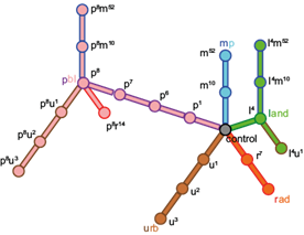
All runs are forced by ERA5 reanalysis (Hersbach et al., 2017) at spatial and temporal resolutions of 30 km and 3 h, respectively. The control simulation (c) uses the following schemes: Mellor-Yamada-Janjic for PBL, Eta similarity for surface layer, Noah for land surface, Thompson for microphysics, RRTMG for radiation, and no urban canopy. Other configurations were selected by changing one scheme at a time as shown in Table I and Figure S1 of the supplementary material. Included PBL schemes are: p1: Yonsei University (YSU, Hong et al., 2006), p2: Mellor- Yamada-Janjic (MYJ, Janjić, 1994), p6: Mellor-Yamada Nakanishi Niino (MYYN, Nakanishi and Niino, 2006), p7: Asymmetric Convection Model 2 Scheme (ACM2, Pleim, 2007), and p8: Bougeault-Lacarrere Scheme (Bougeault and Lacarrere, 1989). Included surface layer schemes: s1: Revised MM5 (Jiménez et al., 2012), s2: Eta Similarity (Janjić, 1994), s5: MYNN and s7: Pleim-Xiu (Pleim, 2006). Included land surface schemes are: l2: Unified Noah Land Surface Model (Noah, Tewari et al., 2004) and l4: Noah-MP Land Surface Model (Noah-Mp, Niu et al., 2011). Included radiation schemes are: r4: RRTMG (Iacono et al., 2008), r7: Fu-Liou-Gu (Gu et al., 2011), and r14: RRTMG-K (Baek, 2017). Included microphysics schemes: m10: Morrison 2-moment (Morrison et al., 2009), and m52: P3 (Morrison and Milbrandt, 2015). Included urban schemes: u1: Urban Canopy Model (Chen et al., 2011), u2: BEP (Martilli et al., 2002), and u3: BEP + BEM (Salamanca et al., 2010).

Table I Model configurations used in the study. 

Label PBL Surface layer Land surface Microphysics Radiation Urban
c MYJ Eta similarity Noah Thompson RRTMG
m10 Morrison 2-moment
m52 P3
r7 Thompson Fu-Liu-Gu
r14 RRTMG-K
u1 RRTMG UCM
u2 BEP
u3 BEP+BEM
p1 YSU Revised MM5
p6 MYNN MYNN
p7 ACM2 Pleim-Xiu
p8 BouLac Revised MM5
p8m10 Morrison 2-moment
p8m52 P3
p8r14 Thompson RRTMG-K
p8u1 RRTMG UCM
p8u2 BEP
p8u3 BEP+BEM
l4 MYJ Eta similarity Noah-MP
l4m10 Morrison 2-moment
l4m52 P3
l4u1 Thompson UCM

As the MABA is a highly urbanized area, an improvement in model performance could be expected with the activation of an urban scheme. For that reason, PBL schemes that are compatible with urban options (in WRF 4.2.1: Mellor-Yamada-Janjic and BouLac) are tested. Although Yonsei University (YSU) and Asymmetric Convection Model 2 (ACM2) are not compatible with the Building Effect Parameterization (BEP) and the Building Energy Model (BEP + BEM) urban schemes in the WRF version used in this work, these are still included as they are widely used in similar studies for air quality applications (e.g., Cuchiara et al., 2014; Banks and Baldasano, 2016; Mohan and Gupta, 2018). BEP (Salamanca and Martilli, 2010) is a 3D urban canopy model which accounts for multiple building parameters allowing for higher constructions than the first model level. BEP + BEM (Martilli et al., 2002) is a multilayer building energy model composed of a building energy model coupled to BEP. BEM accounts for the impacts of anthropogenic heat emissions on the urban environment and estimates the cooling/heating energy demand due to air-conditioning systems. When a UCM is not used, the Noah and Noah-MP LSMs use the Bulk scheme to represent the urban surface in the WRF model. Although the PBL, urban, and land surface model schemes are expected to have a greater impact on model results, we analyze the sensitivity to other physics options (such as radiation and microphysics) as this is the first exploratory study of this kind in the area and these can also affect model performance as found in other works (e.g., Borge et al., 2008).

2.2 Domain

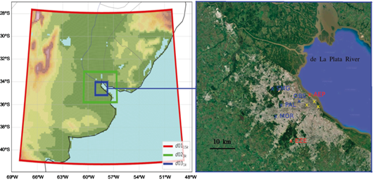
The MABA is composed of the city of Buenos Aires and 24 districts of greater Buenos Aires. It has a population of around 15 million inhabitants over 3800 km2 (INDEC, 2010) of flat terrain and it is surrounded by non-urban areas and the La Plata River on its east side. It is the third most populated megacity in Latin America (UN, 2019). Three modeling nested domains with resolutions of 15 km (111 × 101 grid points), 3 km (121 × 101 grid points), and 1 km (133 × 127 grid points) (Fig. 1) are used with the outermost domain (d01) comprising the whole Buenos Aires province and the innermost domain (d03) covering the whole MABA. Eighty terrain-following hybrid vertical levels near the ground are used. Twelve of them cover the lowest 3 km from the surface with the first level at 24 m. Land uses for this region come from satellite data (Moderate Resolution Imaging Spectroradiometer [MODIS] at a 30” horizontal resolution). Unfortunately, there is only one urban class available for the area at the moment of this study.

Fig. 1 WRF modeling nested domains (left) and map of the MABA (right) with the meteorological (red crosses and blue crosses) and air quality (yellow crosses) stations. Source: Google Maps. 

2.3 Period

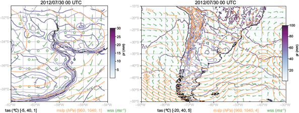
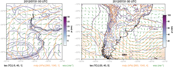
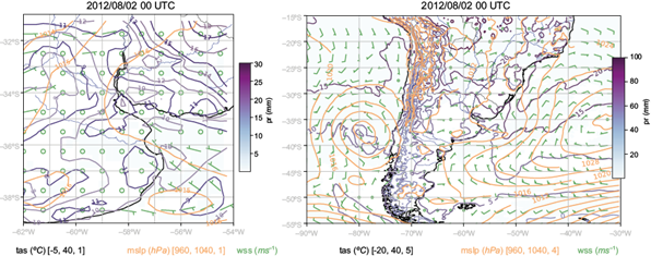
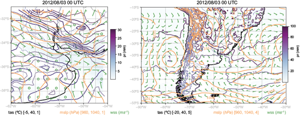
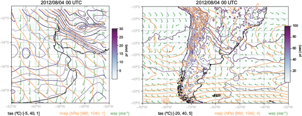
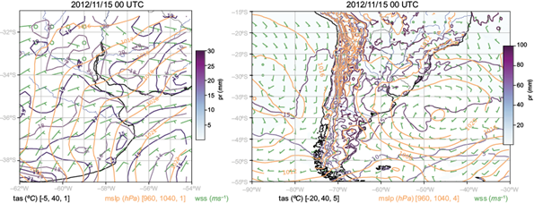
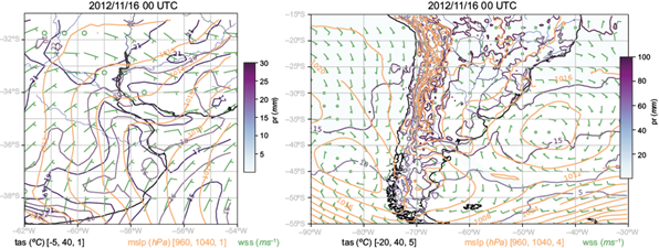
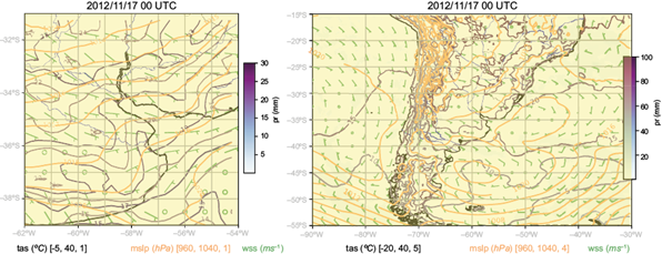
One week in winter and one week in spring of 2012 were chosen to cover different meteorological conditions with enough available data on air pollutants concentration for future air quality model performance validation studies. The first two days of each period are considered as a spin-up. The winter week (July 28 to August 4) started with a high-pressure anomaly on the Atlantic Ocean and a low-pressure anomaly on the Pacific Ocean. This led to a rotation of wind direction and the week ended with precipitation. On the other hand, on the spring period (November 10 to 17) there was a high-pressure disturbance that lasted the whole week with mostly southeastern winds and dry air over the city, as discussed in Luque et al. (2021). Synoptic maps are provided in the supplementary material. All dates presented in this work are expressed in UTC time while the MABA has a local time of UTC-3.

2.4. Model performance evaluation

To assess model performance, four meteorological variables that are relevant for air quality purposes are considered (Ziomas et al., 1995; Harkey et al., 2015): 2-m temperature (T) and water vapor mixing ratio (Qv), and 10-m wind speed (Ws) and direction (Wd). Modeled values of T, Qv, Ws, and Wd are statistically compared with those observed in the Aeroparque meteorological station (AEP, see Fig. 1). This station is the closest one to the three available air quality stations whose data will be used for validation of future air quality simulations and the most representative one. The following statistics are computed: bias, mean absolute error (Mae), root mean square error (Rmse), Correlation (Corr), and index of agreement (Indexagr2) (Emery et al., 2001). This last metric is calculated as the ratio between the Rmse and the sum of the difference between each prediction and the observed mean, and the difference between each observation and the observed mean. It is a measure of the match between the departure of each prediction and each observation from the observed mean. Configurations with the lowest errors and higher Corrs and Indexagr2 are selected to be further analyzed.

For these configurations, the relationship between errors in Wd and Ws is studied following the methodology by Jiménez and Dudhia (2013). In addition, the planetary boundary layer height (PBLH) is explored. PBLH results are contrasted with observations from sounding data available only at 12:00 UTC taken in the Ezeiza Meteorological station (EZE, see Fig. 1). In order to compare PBLH results obtained from the different configurations, modeled and observed values are recalculated following the methodology described in Nielsen-Gammon et al. (2008) and used in other works (e.g., Miao et al., 2022; Yan et al., 2022). This method estimates the PBLH as the height where a “critical inversion occurs”. This height is defined in Marsik et al. (1995) as the level where potential temperature is 1.5 K higher than the minimum value it presents in the PBL.

In order to assess model performance throughout the whole MABA domain, performance metrics are then computed at other meteorological stations for the best performing configurations, which are presented in the supplementary material.

3. Results

3.1 Hourly evolution

Figure 2 presents the hourly evolution of modeled and observed values of Ws, Wd, T, and Qv. Observed Ws values vary between 0 and 10 m s-1, with the lowest ones taking place during the winter week (Fig. 2a, b). Temporal variations for this variable are different between each week and most configurations follow these patterns except for those with complex urban schemes (u2, u3, and p8u3) that show lower wind intensities. During winter week winds come mostly from the SE and SW except for July 31 and August 2, when they come from the NE and N, with very low intensities (Fig. 2c). During the spring week, winds come mostly from the SE (Fig. 2d). This variable is also quite well reproduced by most configurations during both weeks.

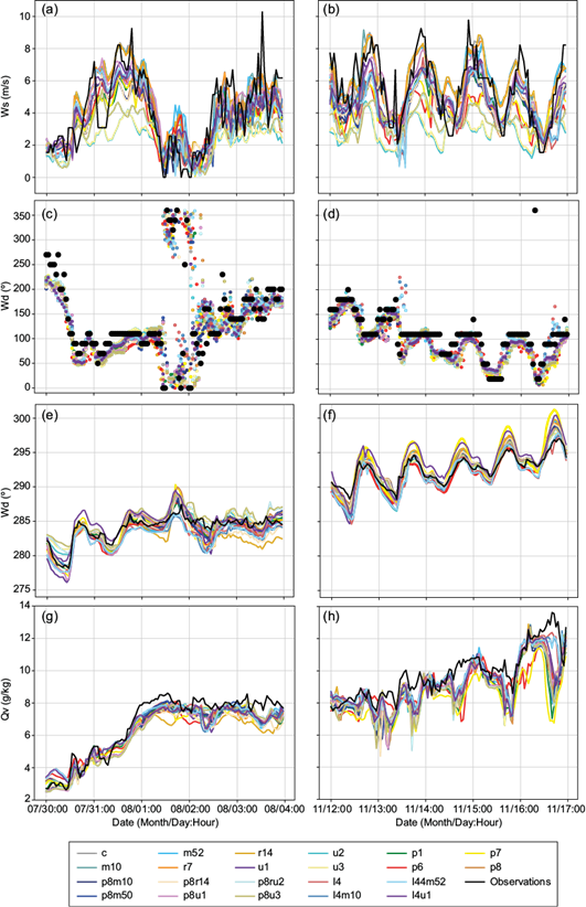
Fig. 2 Temporal evolution of modeled and observed wind speed (Ws [m s-1]), direction (Wd [º]), temperature (T [K]) and vapor mixing ratio [Qv, g kg-1] during winter (left column) and spring (right column) weeks. Hours are written in UTC and the MABA has a local hour of UTC-3. (a) and (b) Ws, (c) and (d) Wd, (e) and (f) T, (g), and (h) Qv. 

Observed T values (Fig. 2e, f) display different behaviors between the two periods, with a clearer diurnal cycle during spring. Most configurations follow observations, even though for some of them differences tend to become larger over time showing the expected decrease in model skill as time of forecast increases (Buizza and Leutbecher, 2015).

During the winter week, observed values of Qv rapidly grow until August 1 (Fig. 2g), when precipitation starts reaching its maximum value. This behavior is due to the fact that on July 31 there is a high-pressure zone in front of the coastline of Uruguay centered around 35º S and 55º W (see Figs. S2 to S7 in the supplementary material). The circulation associated with the high-pressure anomaly advects wetter air towards the Buenos Aires area. After that, variations are smaller. During the spring week, an increase in Qv is also seen (Fig. 2h). During both periods, all simulations reproduce well the time evolution of Qv but underestimate its values between -16 and -5% depending on the configuration, mainly in spring.

3.2 Performance metrics

In order to select the best performing configurations, Figure 3 presents the bias, Mae, Rmse, Corr and Indexagr2 computed for each variable, week and configuration. For values of each statistic see section S3 in the supplementary material. For Ws, configurations present similar performance metrics during both weeks (Fig. 3a), but relative error values are smaller in spring (not shown). Relatively large values of Corr (> 0.77) and Indexagr2 (> 0.88) are obtained for most schemes. Configurations with complex urban schemes (which include the label u2 or u3: u2, u3, p8u2, and p8u3) present the worst performance metrics with Mae 20-30% higher than the other configurations and lower Correlations, specially u2 and u3 during the spring week, which present Correlation values below 0.3. While a better performance with these configurations could be expected in the highly urbanized MABA, some works show that complex urban schemes behave better when local urban parameters suited for the particular city under study are used (e.g., Kuik et al., 2016; Shen et al., 2019). In this first stage of the model implementation, default WRF urban parameters are used. A sensitivity test to the multiple parameters (e.g., building height and albedo, among others) used to configure the urban schemes is beyond the scope of this work due to computational constraints and the lack of a set of available reference values for these parameters in MABA. The larger underestimation for this variable obtained with configurations with BEP and BEP + BEM (u2, u3, p8u2, and p8u3) could be due to an overestimation of the urban fraction in AEP as a consequence of using default urban parameters. The other configurations without complex urban schemes present bias, Mae and Rmse in the ranges of -1.6 to 0.5 m s-1 (with relative values of -28.2 to 1.3%), 0.9 to 1.8 m s-1 (17.6 to 33.2%), and 1.5 to 2.1 m s-1 (27.7 to 53.2%), respectively. During both weeks, configurations with a simple urban scheme (those labelled with u1, p8u1 and l4u1) have the lowest errors. In the spring, p8u1 has the best performance as it also presents the higher Corr and Indexagr2.

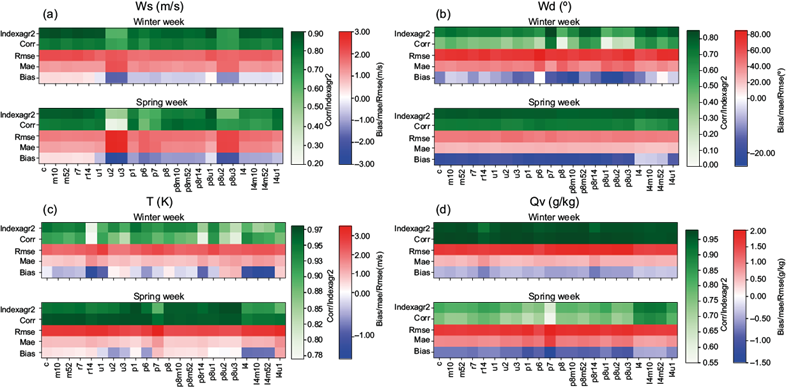
Fig. 3 Statistics (vertical axis) for Ws (m s-1), Wd (º), T (K) and Qv (g kg-1) for both weeks and all configurations (horizontal axis). Index of agreement and Correlation in green and errors in red, white and blue. (a) Ws, (b) Wd, (c) T, and (d) Qv. 

Wd (Fig. 3b) is counter-clockwise biased by almost all configurations during both periods with bias ranging between -23.4º and -4.2º (-16.6 and -2.9% with stronger underestimations during spring), Mae between 18.7º-52.2º (17.0-37.0%) and Rmse in the range 40.9º-75º (37.2-53.4%). During the winter week, Mae and Rmse values are relatively higher. The configuration with the MYNN PBL scheme (p6) has a bias close to 0% but this is clearly due to a compensation of errors in the calculation, as this configuration also has the highest Rmse and Mae. Both Corr and Indexagr2 are higher during the spring with values greater than 0.6. Configurations with the Noah-MP land surface scheme (l4, l4m10 and l4m52), with the exception of the combination with the simple urban scheme (l4u1), have clearly the lowest errors during both weeks with similar Corr and Indexagr2 to those of other configurations.

For T (Fig. 3c), Corr and Indexagr2 are higher during the spring week than during the winter week with values above 0.9. This is expected as a better representation of the diurnal cycle is observed in the spring period (Fig. 2e, f). Still, all Corr and Indexagr2 have values over 0.7 in the winter week. For both periods, bias, Mae and Rmse values range from -1.4 to 1.2 K (-0.5-0.4%), 0.5 K to 1.5 K (0.2-0.5%) and 1.8K to 3.4 K (0.6-1.2%) respectively. Configurations with Noah-Mp land surface scheme without urban scheme (l4, l4m10 and l4m52) slightly underestimate T while the only configuration with Noah-Mp and urban scheme (l4u1) overestimates it. This is most likely due to the activation of the urban scheme. Other configurations share this characteristic and do not exhibit a similar positive bias, but they also have a different land surface model (u1) and a different PBL scheme (p8u1). The use of urban schemes improves the performance during the spring week, but not during the winter one. A possible explanation for this is that the impact of urban environments is larger during the nocturnal period, when the impact of accumulated heat from buildings and paved surfaces is more noticeable (Argüeso et al., 2014). Therefore, it is expected that the impact of the presence of urban structures would be more noticeable during the warmer season, when the solar radiation is also more abundant.

Qv is underestimated during both weeks, as observed in Figure 2g, h with bias values in the range of -1.1 and -0.3 g kg-1 (-4.65 and -1.39%) (Fig. 3d). Mae and Rmse are both in the range of 1.3-2.5 g kg-1. Corr and Indexagr2 are higher in the winter week than in the spring one with values over 0.9. During the spring period, on the other hand, Corr and Indexagr2 values are close to 0.7 with the exception of configurations with Noah-Mp (l4, l4m10 and l4m52), which have similar values to those obtained in the winter week, and p7, that presents lower values than other configurations.

In order to gain preliminary insight on the impact of each physical scheme on surface meteorological variables, configurations that share all characteristics except one are compared: c (control run), m10, and m52 differ only in their microphysics scheme (Thompson, Morrison 2-moment, and P3, respectively) and as can be seen in Figure 3, the four configurations present similar behavior, suggesting that this scheme does not significantly affect the model performance. The same is observed with the radiation scheme, as configurations c, r7 and r14 differ only in their microphysics scheme (RRTMG, Fu-Liu-Gu, and RRTMG-K, respectively) and they present similar results.

Configurations c, u1, u2 and u3 differ only in their urban scheme (Bulk scheme, simple layer, BEP, and BEP + BEM, respectively). Contrary to what happens with the microphysics and radiation parametrizations, here we see a clear effect. Results of the three configurations with urban schemes (u1, u2, and u3) change mostly in the case of Ws, giving lower values than the control configuration due to the increase in surface roughness length and blocking effects associated to buildings. They also affect results for T. Contrary as expected, the activation of the urban scheme lowers its values during both weeks.

Configurations c, p1, p6, p7, and p8 differ on their PBL and surface scheme (MYJ + Eta similarity, MYNN, ACM2+Pleim, Xiu and BouLac + Revised MM5, respectively). Control simulation differs from the others with higher Ws and T values, but these subsets of simulations behave similarly. The exception is p7, which has a better performance for Wd during the winter week, but a lower one for Qv and T during the spring week.

Lastly, configurations c and l4 differ only in their land surface model (Noah for c and Noah MP for l4). Therefore, minimum differences are expected between the results obtained with both configurations at an urban grid cell such as AEP; however, l4 shows a slight improvement in the representation of Qv and Wd compared with c, especially during the spring week. A possible explanation for this is that since both variables depend on their values in other cells, an impact from remote non-urban cells could be affecting the results found in AEP.

These comparisons suggest that the urban scheme has a greater influence on the model performance while radiation and microphysics schemes have a negligible effect. However, since the response to different physical schemes is not linear, more configurations should be compared with each other at more weather stations to have a clearer conclusion regarding this matter.

Almost all configurations have good performances for T and Qv. This is consistent with previous works where the dynamics of these variables are easier to represent by the model than Ws and Wd (e.g., Cuchiara et al., 2014; Banks and Baldasano, 2016; Mohan and Gupta, 2018). For this reason, the selection of configurations for further inspection is based on model performance to estimate the wind variables.

It should be noted that while Wd is mostly influenced by synoptic/mesoscale conditions, Ws can also be influenced by local dynamics that depend on model configuration. This could explain that while dynamics of the predominant synoptic/mesoscale features might not be too different between simulations, the wind intensity might be. The best performance to estimate Ws and l4 is given by l4m10, while l4m52 presents the best performance for Wd. Configurations p1 and l4u1 are also selected to analyze the impact of different PBL schemes (a local scheme and a non-local one, respectively) and whether the activation of a simple urban scheme plays a role in performance.

Figure 4 shows the differences between hourly observed and modeled values for all variables in each of the six configurations. For Ws, most differences are within the range -2-2 m s-1 and behave similarly among configurations (Fig. 4a, b). During both weeks, p8u1 usually presents slightly higher Ws values than the rest (typically by 1 m s-1, which represents around 25 or 17% of the observed mean, depending on the week). This leads to a somewhat larger overestimation of minimums but a smaller underestimation of maximums. On the other hand, p1 (configured with YSU as PBL scheme) presents lower Ws values (around 1 m s-1); therefore, it overestimates less minimums values, but underestimates more maximums values. Configurations with Noah-Mp are an intermediate case. During some periods of a few hours, the difference between model results and observations are larger than 2 m s-1, which represents around 34 or 50% of the observed mean depending on the week. For all configurations, the largest underestimation (6 m s-1) coincides with the global observed maximum of Ws (see Fig. 2a).

Fig. 4 Differences between modeled values of Ws (m s-1), Wd (º), T (K) and Qv (g kg-1) with observations for chosen configurations for the winter (left column) and spring week (right column). The range in which most differences lie is colored in grey. (a) and (b) Ws, (c) and (d) Wd, (e) and (f) T, (g) and (h) Qv. 

Differences between modeled and observed Wd values for the different configurations are also similar to each other and within the range -50-50º (Fig. 4c, d). Larger differences are observed around August 2 at 00:00 UTC when Ws values are close to 0 m s-1 and the midday of November 13 and 16, when configurations with Noah-MP predict Ws values lower than 2 m s-1.

In the case of T (Fig. 4e, f), most differences with observations are in the range -2 to 2 K but larger differences among the selected configurations are observed, compared to those of wind variables. During both weeks, l4u1 shows larger (and mainly positive) differences between modeled and observed T values, while best performing schemes for Wd (l4, l4m10, and l4m52) present lower (and mostly negative) differences, as also shown in Figure 4c. During the spring week, l4u1 shows a larger overestimation of temperature, which increases with time during the last three days of the period. On the other hand, configurations p1 and p8u1 usually present smaller differences. To understand why configuration l4u1 (Noah-Mp + single layer urban scheme) overestimates observations and presents values between 1 and 4 K higher than the others, surface heat fluxes are explored (see section S4 in the supplementary material). A higher sensible heat flux for this configuration (l4u1) is expected, but it is found that it presents values similar to the other, all with higher values during the spring week. To understand why it still presents higher T, surface temperature is analyzed, since sensible heat flux depends on the temperature difference between the surface and the air above it. If surface temperature is higher in this configuration, it could explain why it presents similar sensible heat values as the other configurations, but with a higher T. This is the case, and is most likely due to the activation of the urban scheme.

For Qv (Fig. 4g, h), differences between model results and observations are mostly negative and vary similarly. During the winter week, most differences range between -1.5 and 1.0 g kg-1. Configurations p1 and p8u1 present larger differences with observations, especially during the spring week where a greater underestimation (up to 6 g kg-1) is observed. From Figure 2h, it can be seen that in this week the largest underestimations occur around minimums.

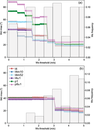
To better understand the relationship between wind direction errors and wind speed, the root mean square error of Wd is calculated for different subsets of data, eliminating those with observed Ws values below a given threshold, which varies between 0 and 5 m s-1 covering most of the dataset in order to find if a change in behavior exists at some point and how configurations behave after it. This is done for the six selected configurations (Fig. 5). Rmse for all configurations in both weeks is larger for lower Ws threshold values, consistent with results by Jiménez and Dudhia (2013). During the winter week (Fig. 5a), the Wd Rmse varies from 44º to 18º for Noah-Mp configurations, 73º to 20º for p1, and 88º to 24º for p8u1. A very small variation of Wd Rmse is observed for Ws threshold values above 2.6 m s-1. The most abrupt decrease (70%) is presented by p8u1, highlighting its large sensitivity to this variable for low Ws values. Note that around 35% of wind speed measurements during this week have wind speed values below 2.6 m s-1. In turn, during the spring week (Fig. 5b), the Wd Rmse varies form 38º to 19º, representing a change of around 40%) for all configurations. This change in Rmse occurs when the threshold is around 3.1 m s-1. In this case, only 19% of the observed hourly Ws values are below this value. The larger presence of lighter winds during the winter week may explain the relatively worse results to simulate wind variables during this period.

Fig. 5 Wd (º) Rmse (left side scale) for different Ws (m s-1) threshold and Ws frequency (m s-1) (right side scale) for different wind speed values. Filled light grey bars show the normalized probability density function for observed Ws. (a) Winter week, (b) spring week. 

3.3. Planetary boundary layer height

Figure 6 shows modeled PBLH values at AEP and EZE stations (Fig. 1) during both weeks. Only five sounding data points are available for EZE (black dots) during the analyzed period, and they are included only for comparison in the EZE plots. For each week, the temporal variations of the PBLH are similar at the two stations, with maximum diurnal values being somewhat higher at AEP. At these sites, modeled PBLH values vary from 100 to 1500 m during the winter week and from 250 to 2000 m in the spring week. These values are a bit higher than the ones studied in Mazzeo and Gassmann (1990), who found average maximum values of 1100 m during August and 1500 m during November. In general, configurations present similar temporal variations with higher PBLH values during the day and lower ones at nighttime, as expected. However, large differences are observed on some days. For example, on July 31, p8u1 presents larger values than other configurations at the two stations. This is consistent with the fact that this configuration also presents higher wind speed values leading to more mechanical turbulence during that day. On November 16 and 17, p8u1 and p1 simulate PBLH peaks that are considerably higher (by 1000 m) than those estimated by other configurations. Although on November 17 p1 and p8u1 present stronger wind intensities that could partially explain this, no significant differences in wind speed between configurations are observed on November 16.

Fig. 6 Planetary boundary layer height for chosen configurations and observations (black dots) for winter (left column) and spring weeks (right column). (a) and (b) Aeroparque, (c) and (d) Ezeiza. 

3.4. Performance evaluation at other meteorological stations

Model performances metrics (bias, Mae, Rmse, Corr and Indexagr2) are computed for best performing configurations for Ws and Wd at AEP (p8u1 and l4, respectively) at other five meteorological stations of the MABA (San Miguel [SMG], Ezeiza [EZE], Moron [MOR], Observatorio de Buenos Aires [OBS] and Palomar [PAL]; see Fig. 1). Results are included in section S5 in the supplementary material. Both configurations present a good performance to estimate T with Corr > 0.7 and errors under 15% for all stations. Similar results are obtained for Qv with the exception of San Miguel and Moron stations during the spring week. On the other hand, model performance to estimate Ws and Wd varies with the station and the week. Ws presents an acceptable performance (Corr > 0.6 and Mae < 35%) in Ezeiza and Palomar stations during both weeks and in Moron during the spring period, but a poor one in San Miguel and Palomar during the winter week. Wd has an acceptable performance in Ezeiza and in Moron during the winter period. The worst model performance for both wind variables is obtained at OBS, which may be expected as this station is surrounded by buildings and trees that affect wind measurements (Mazzeo and Gassmann, 1990).

4. Conclusions

The performance of the WRF model to simulate wind speed (Ws), wind direction (Wd), air temperature (T) and water vapor mixing ratio (Qv) in the Metropolitan Area of Buenos Aires (MABA) under different parameterizations of the physical processes in the PBL is analyzed. It is found that there is no single configuration that presents the best performance for all variables. This is consistent with previous works performed for other urban areas. Ws is mostly affected by the activation of a simple urban scheme, especially during the spring week, and model performance is improved when coupled with the BouLac PBL. On the other hand, Wd and Qv are most sensitive to changes in the land surface scheme. For both variables, performance improves when using Noah-MP, especially during the spring week. The ability of WRF to estimate T improves with the activation of the urban and the BouLac PBL schemes during the spring week, but not during the winter. On the other hand, when the simple urban scheme is coupled with Noah-Mp land surface model, T values are consistently higher than for any other configuration and overestimate observations.

In general, the selected configurations present similar hourly evolutions of the PBLH values, but some configurations have significantly higher values during certain days, which can be explained by the fact that they also exhibit higher wind intensities that might produce higher mechanical turbulence.

In the Aeroparque (AEP) station and for the surface variables analyzed in this work, configurations with Noah-Mp land surface model scheme and the combination of BouLac PBL with the simple urban scheme, show the best overall performance during the analyzed weeks. They reproduce both T and Qv relatively well (with Mae lower than 1 and 10%, respectively) and present the best performance: Noah-Mp for Wd (Mae < 25%) and Boulac coupled with a simple urban scheme for Ws (Mae < 28%). For all variables, these configurations present Corr over 0.7.

Overall, performance for T and Qv is acceptable at all meteorological stations, while p8u1 and l4 perform best for wind variables at the AEP meteorological station, though they show poor results at some other sites of the MABA. Future work including local information on urban parameters (as they become available) will allow to study whether more complex urban schemes (BEP and BEP + BEM) can improve model performance at those stations.

Acknowledgments

The authors are grateful to the Servicio Meteorológico Nacional (SMN) for providing the meteorological data. This work has been funded by Project PICT2018-1624 from the Agencia Nacional de Promoción Científica y Tecnológica (ANPCyT). Simulations were performed on the HPC resources of CIMA, a member of the National High-Performance Computing System (SCAD).

References

Argüeso D, Evans JP, Fita L, Bormann KJ. 2014. Temperature response for future urbanization and climate change. Climate Dynamics 42: 2183-2199. https://doi.org/10.1007/s00382-013-1789-6 [ Links ]

Baek S. 2017. A revised radiation package of G-packed McICA and two-stream approximation: Performance evaluation in a global weather forecasting model. Journal of Advances in Modeling Earth Systems 9: 1628-1640. https://doi.org/10.1002/2017MS000994 [ Links ]

Banks RF, Baldasano JM. 2016. Impact of WRF model PBL schemes on air quality simulations over Catalonia, Spain. Science of The Total Environment 572: 98-113. https://doi.org/10.1016/j.scitotenv.2016.07.167 [ Links ]

Borge R, Alexandrov V, del Vas JJ, Lumbreras J, Rodríguez E. 2008. A comprehensive sensitivity analysis of the WRF model for air quality applications over the Iberian Peninsula. Atmospheric Environment 42: 8560-8574. https://doi.org/10.1016/j.atmosenv.2008.08.032 [ Links ]

Bougeault P, Lacarrere P. 1989. Parameterization of orography-induced turbulence in a mesobeta-scale model. Monthly Weather Review 117: 1872-1890. https://doi.org/10.1175/1520-0493(1989)117<1872:POOITI>2.0.CO;2 [ Links ]

Buizza R, Leutbecher M. 2015. The forecast skill horizon. Quarterly Journal of the Royal Meteorological Society 141: 3366-3382. https://doi.org/10.1002/qj.2619 [ Links ]

Chen F, Kusaka H, Bornstein R, Ching J, Grimmond CBS, Grossman-Clarke S, Loridan T, Manning KW, Martilli A, Miao S, Sailor D, Salamanca FP, Taha H, Tewari M, Wang X, Wyszogrodzki AA, Zhang C. 2011. The integrated WRF/urban modelling system: Development, evaluation, and applications to urban environmental problems. International Journal of Climatology 31: 273-288. https://doi.org/10.1002/joc.2158 [ Links ]

Cheng FY, Feng CY, Yang ZM, Hsu CH, Chan KW, Lee CY, Chang SC. 2021. Evaluation of real-time PM2.5 forecasts with the WRF-CMAQ modeling system and weather-pattern-dependent bias-adjusted PM2.5 forecasts in Taiwan. Atmospheric Environment 244: 117909. https://doi.org/10.1016/j.atmosenv.2020.117909 [ Links ]

Cogliani E. 2001. Air pollution forecast in cities by an air pollution index highly correlated with meteorological variables. Atmospheric Environment 35: 2871-2877. https://doi.org/10.1016/S1352-2310(01)00071-1 [ Links ]

Cuchiara GC, Li X, Carvalho J, Rappenglück B. 2014. Intercomparison of planetary boundary layer parameterization and its impacts on surface ozone concentration in the WRF/Chem model for a case study in Houston/Texas. Atmospheric Environment 96: 175-185. https://doi.org/10.1016/j.atmosenv.2014.07.013 [ Links ]

De la Paz D, Borge R, Martilli A. 2016. Assessment of a high resolution annual WRF-BEP/CMAQ simulation for the urban area of Madrid (Spain). Atmospheric Environment 144: 282-296. https://doi.org/10.1016/j.atmosenv.2016.08.082 [ Links ]

Emery C, Tai E, Yarwood G. 2001. Enhanced meteorological modeling and performance evaluation for two Texas ozone episodes. Texas Natural Resource Conservation Commission, Austin, TX. [ Links ]

Evans JP, Ekström M, Ji F. 2012. Evaluating the performance of a WRF physics ensemble over South-East Australia. Climate Dynamics 39: 1241-1258. https://doi.org/10.1007/s00382-011-1244-5 [ Links ]

Gaur A, Lacasse M, Armstrong M, Lu H, Shu C, Fields A, Palou FS, Zhang Y. 2021. Effects of using different urban parametrization schemes and land-cover datasets on the accuracy of WRF model over the City of Ottawa. Urban Climate 35: 100737. https://doi.org/10.1016/j.uclim.2020.100737 [ Links ]

Harkey M, Holloway T, Oberman J, Scotty E. 2015. An evaluation of CMAQ NO2 using observed chemistry-meteorology correlations. Journal of Geophysical Research: Atmospheres 120: 11775-11797. https://doi.org/10.1002/2015JD023316 [ Links ]

Hersbach H, Bell B, Berrisford P, Hirahara S, Horányi A, Muñoz-Sabater J, Nicolas J, Peubey C, Radu R, Schepers D, Simmons A, Soci C, Abdalla S, Abellan X, Balsamo G, Bechtold P, Biavati G, Bidlot J, Bonavita M, De Chiara G, Dahlgren P, Dee D, Diamantakis M, Dragani R, Flemming J, Forbes R, Fuentes M, Geer A, Haimberger L, Healy S, Hogan RJ, Hólm E, Janisková M, Keeley S, Laloyaux P, Lopez P, Lupu C, Radnoti G, de Rosnay P, Rozum I, Vamborg F, Villaume S, Thépaut J-N. 2017. Complete ERA5 from 1940: Fifth generation of ECMWF atmospheric reanalyses of the global climate. Copernicus Climate Change Service (C3S) Data Store (CDS). https://doi.org/10.24381/cds.143582cf [ Links ]

Gu Y, Liou KN, Ou SC, Fovell R. 2011. Cirrus cloud simulations using WRF with improved radiation parameterization and increased vertical resolution. Journal of Geophysics Research: Atmospheres 116: D06119. https://doi.org/10.1029/2010JD014574 [ Links ]

Hong SY, Noh Y, Dudhia J. 2006. A new vertical diffusion package with an explicit treatment of entrainment processes. Monthly Weather Review 134: 2318-2341. https://doi.org/10.1175/MWR3199.1 [ Links ]

Huang Y, Guo B, Sun H, Liu H, Chen SX. 2021. Relative importance of meteorological variables on air quality and role of boundary layer height. Atmospheric Environment 267: 118737. https://doi.org/10.1016/j.atmosenv.2021.118737 [ Links ]

Iacono MJ, Delamere JS, Mlawer EJ, Shephard MW, Clough SA, Collins WD. 2008. Radiative forcing by long-lived greenhouse gases: Calculations with the AER radiative transfer models. Journal of Geophysical Research: Atmospheres 113: D13103. https://doi.org/10.1029/2008JD009944 [ Links ]

INDEC. 2010. Censo Nacional de Población, Hogares y Viviendas. Instituto Nacional de Estadística y Censos. Available at: Available at: https://www.indec.gob.ar/indec/web/Nivel4-Tema-2-41-135 (accessed 2022 March 13). [ Links ]

Janjić ZI. 1994. The Step-Mountain Eta Coordinate Model: Further developments of the convection, viscous sublayer, and turbulence closure schemes. Monthly Weather Review 122: 927-945. https://doi.org/10.1175/1520-0493(1994)122<0927:TSMECM>2.0.CO;2 [ Links ]

Jia W, Zhang X. 2020. The role of the planetary boundary layer parameterization schemes on the meteorological and aerosol pollution simulations: A review. Atmospheric Research 239: 104890. https://doi.org/10.1016/j.atmosres.2020.104890 [ Links ]

Jiménez PA, Dudhia J, González-Rouco JF, Navarro J, Montávez JP, García-Bustamante E. 2012. A revised scheme for the WRF surface layer formulation. Monthly Weather Review 140: 898-918. https://doi.org/10.1175/MWR-D-11-00056.1 [ Links ]

Jiménez PA, Dudhia J. 2013. On the ability of the WRF model to reproduce the surface wind direction over complex terrain. Journal of Applied Meteorology and Climatology 52: 1610-1617. https://doi.org/10.1175/JAMC-D-12-0266.1 [ Links ]

Kitagawa YKL, de Almeida Albuquerque TT, Kumar P, Nascimento EGS, Moreira DM. 2022. Coastal-urban meteorology: A sensitivity study using the WRF-urban model. Urban Climate 44: 101185. https://doi.org/10.1016/j.uclim.2022.101185 [ Links ]

Kuik F, Lauer A, Churkina G, Denier van der Gon HAC, Fenner D, Mar KA, Butler TM. 2016. Air quality modelling in the Berlin-Brandenburg region using WRF-Chem v3.7.1: Sensitivity to resolution of model grid and input data. Geoscientific Model Development 9: 4339-4363. https://doi.org/10.5194/gmd-9-4339-2016 [ Links ]

Liao J, Wang T, Wang X, Xie M, Jiang Z, Huang X, Zhu J. 2014. Impacts of different urban canopy schemes in WRF/Chem on regional climate and air quality in Yangtze River Delta, China. Atmospheric Research 145-146: 226-243. https://doi.org/10.1016/j.atmosres.2014.04.005 [ Links ]

Luque SE, Fita L, Rojas ALP. 2021. WRF model set-up analysis for air quality simulations in the Metropolitan Area of Buenos Aires. In: Proceedings of the 2021 Congreso Colombiano y Conferencia Internacional de Calidad de Aire y Salud Pública (CASAP), Bogotá, Colombia. https://doi.org/10.1109/CASAP54985.2021.9703379 [ Links ]

Marsik FJ, Fischer KW, McDonald TD, Samson PJ. 1995. Comparison of methods for estimating mixing height used during the 1992 Atlanta Field Intensive. Journal of Applied Meteorology and Climatology 34: 1802-1814. https://doi.org/10.1175/1520-0450(1995)034<1802:COMFEM>2.0.CO;2 [ Links ]

Martilli A, Clappier A, Rotach MW. 2002. An urban surface exchange parameterisation for mesoscale models. Boundary-Layer Meteorology 104: 261-304. https://doi.org/10.1023/A:1016099921195 [ Links ]

Mazzeo NA, Gassmann MI. 1990. Mixing heights and wind direction analysis for urban and suburban areas of Buenos Aires city. Energy and Buildings 3-4: 333-337. https://doi.org/10.1016/0378-7788(90)90006-5 [ Links ]

Miao Y, Liu S, Huang S. 2019. Synoptic pattern and planetary boundary layer structure associated with aerosol pollution during winter in Beijing, China. Science of The Total Environment 682: 464-474. https://doi.org/10.1016/j.scitotenv.2019.05.199 [ Links ]

Miao Y, Che H, Liu S, Zhang X. 2022. Heat stress in Beijing and its relationship with boundary layer structure and air pollution. Atmospheric Environment 282: 119159. https://doi.org/10.1016/j.atmosenv.2022.119159 [ Links ]

Mohan M, Gupta M. 2018. Sensitivity of PBL parameterizations on PM10 and ozone simulation using chemical transport model WRF-Chem over a sub-tropical urban airshed in India. Atmospheric Environment 185: 53-63. https://doi.org/10.1016/j.atmosenv.2018.04.054 [ Links ]

Morrison H, Thompson G, Tatarskii V. 2009. Impact of cloud microphysics on the development of trailing stratiform precipitation in a simulated squall line: Comparison of one- and two-moment schemes. Monthly Weather Review 137: 991-1007. http://doi.org/10.1175/2008MWR2556.1 [ Links ]

Morrison H, Milbrandt JA. 2015. Parameterization of cloud microphysics based on the prediction of bulk ice particle properties. Part I: Scheme description and idealized tests. Journal of the Atmospheric Sciences 72: 287-311. https://doi.org/10.1175/JAS-D-14-0065.1 [ Links ]

Nakanishi M, Niino H. 2006. An improved Mellor-Yamada level-3 model: Its numerical stability and application to a regional prediction of advection fog. Boundary-Layer Meteorology 119: 397-407. https://doi.org/10.1007/s10546-005-9030-8 [ Links ]

NASEM. 2019. Review of the Bureau of Ocean Energy Management “Air Quality Modeling in the Gulf of Mexico Region” study. National Academies of Sciences, Engineering, and Medicine, Washington, DC. https://doi.org/10.17226/25600 [ Links ]

Nielsen-Gammon JW, Powell CL, Mahoney MJ, Angevine WM, Senff C, White A, Berkowitz C, Doran C, Knupp K. 2008. Multisensor estimation of mixing heights over a coastal city. Journal of Applied Meteorology and Climatology 47: 27-43. https://doi.org/10.1175/2007JAMC1503.1 [ Links ]

Niu GY, Yang ZL, Mitchell KE, Chen F, Ek MB, Barlage M, Kumar A, Manning K, Niyogi D, Rosero E, Tewari M, Xia Y. 2011. The community Noah land surface model with multiparameterization options (Noah-MP): 1. Model description and evaluation with local-scale measurements. Journal of Geophysical Research: Atmospheres 116: D12109. https://doi.org/10.1029/2010JD015139 [ Links ]

Pearce JL, Beringer J, Nicholls N, Hyndman RJ, Tapper NJ. 2011. Quantifying the influence of local meteorology on air quality using generalized additive models. Atmospheric Environment 45: 1328-1336. https://doi.org/10.1016/j.atmosenv.2010.11.051 [ Links ]

Pleim JE. 2006. A simple, efficient solution of flux-profile relationships in the atmospheric surface layer. Journal of Applied Meteorology and Climatology 45: 341-347. https://doi.org/10.1175/JAM2339.1 [ Links ]

Pleim JE. 2007. A combined local and nonlocal closure model for the atmospheric boundary layer. Part I: Model description and testing. Journal of Applied Meteorology and Climatology 46: 1383-1395. https://doi.org/10.1175/JAM2539.1 [ Links ]

Rafael S, Rodrigues V, Fernandes AP, Augusto B, Borrego C, Lopes M. 2019. Evaluation of urban surface parameterizations in WRF model using energy fluxes measurements in Portugal. Urban Climate 28: 100465. https://doi.org/10.1016/j.uclim.2019.100465 [ Links ]

Salamanca F, Krpo A, Martilli A, Clappier A. 2010. A new building energy model coupled with an urban canopy parameterization for urban climate simulations-Part I. formulation, verification, and sensitivity analysis of the model. Theoretical and Applied Climatology 99: 331-344. https://doi.org/10.1007/s00704-009-0142-9 [ Links ]

Salamanca F, Martilli A. 2009. A new Building Energy Model coupled with an Urban Canopy Parameterization for urban climate simulations-Part II. Validation with one-dimension off-line simulations. Theoretical and Applied Climatology 99: 345-356. https://doi.org/10.1007/s00704-009-0143-8 [ Links ]

Shen C, Chen X, Dai W, Li X, Wu J, Fan Q, Wang X, Zhu L, Chan P, Hang J, Fan S, Li W. 2019. Impacts of high-resolution urban canopy parameters within the WRF Model on dynamical and thermal fields over Guangzhou, China. Journal of Applied Meteorology and Climatology 58: 1155-1176. https://doi.org/10.1175/JAMC-D-18-0114.1 [ Links ]

Skamarock WC, Klemp JB, Dudhia J, Gill DO, Liu Z, Berner J, Wang W, Powers JG, Duda MG, Barker D, Huang XY. 2019. A description of the advanced research WRF model version 4.1 NCAR No. NCAR/TN-556+STR Technical Note http://doi.org/10.5065/1dfh-6p97 [ Links ]

Sulaymon ID, Zhang Y, Hu J, Hopke PK, Zhang Y, Zhao B, Xing J, Li L, Mei X. 2021. Evaluation of regional transport of PM2.5 during severe atmospheric pollution episodes in the western Yangtze River Delta, China. Journal of Environmental Management 293: 112827. http s://doi.org/10.1016/j.jenvman.2021.112827 [ Links ]

Tewari M, Chen F, Wang W, Dudhia J, Lemone MA, Mitchell KE, Ek M, Gayno G, Wegiel JW, Cuenca R. 2004. Implementation and verification of the unified Noah land-surface model in the WRF model. In: Proceedings of the 20th Conference on Weather Analysis and Forecasting/16th Conference on Numerical Weather Prediction. American Meteorological Society, Seattle, WA, USA. [ Links ]

UN. 2019. World urbanization prospects: The 2018 revision (st/esa/ser.a/420). United Nations Department of Economics and Social Affairs, Population Division, New York, NY, USA. [ Links ]

Vongruang P, Pimonsree S. 2020. Biomass burning sources and their contributions to PM10 concentrations over countries in mainland southeast Asia during a smog episode. Atmospheric Environment 228: 117414. https://doi.org/10.1016/j.atmosenv.2020.117414 [ Links ]

Yan Y, Cai X, Miao Y, Yu M. 2022. Synoptic condition and boundary layer structure regulate PM2.5 pollution in the Huaihe River Basin, China. Atmospheric Research 269: 106041. https://doi.org/10.1016/j.atmosres.2022.106041 [ Links ]

Zhang Y, Cao S, Zhao L, Cao J. 2022. A case application of WRF-UCM models to the simulation of urban wind speed profiles in a typhoon. Journal of Wind Engineering and Industrial Aerodynamics 220: 104874. https://doi.org/10.1016/j.jweia.2021.104874 [ Links ]

Ziomas IC, Melas D, Zerefos CS, Bais AF, Paliatsos AG. 1995. Forecasting peak pollutant levels from meteorological variables. Atmospheric Environment 29: 3703-3711. https://doi.org/10.1016/1352-2310(95)00131-H [ Links ]

Supplementary material

S1. Model configurations

Figure S1 shows a map of all configurations studied in this work.

Fig. S1 Graphic representation of the multiphysics used in the study. Different options are used for five physics schemes taking as reference the ‘control’ simulation (‘central station’ in black): mp (micro-physics, blue), land (land, green), rad (radiation, red), urb (urban, brown), pbl (boundary layer, pink). Changes in one of the schemes within the map open a new ‘metro’ branch preserving the same direction and color. When two changes are occurring a combination of colors is done. Only l4u1 simulation does not follow the direction rule. 

S2. Synoptic conditions

Figures S2, S3, S4, S5, S6, S7, S8, S9, S10, S11, S12 and S13 present the synoptic conditions for both weeks studied (July 30 to August 4 and November 12 to 17, 2012) over the MABA and Argentina.

Fig. S2 Synoptic map for July 30 at 00:00 UTC over the MABA (left panel) and Argentina (right panel). 

Fig. S3 Synoptic map for July 31 at 00:00 UTC over the MABA (left panel) and Argentina (right panel). 

Fig. S4 Synoptic map for August 1 at 00:00 UTC over the MABA (left panel) and Argentina (right panel). 

Fig. S5 Synoptic map for August 2 at 00:00 UTC over the MABA (left panel) and Argentina (right panel). 

Fig. S6 Synoptic map for August 3 at 00:00 UTC over the MABA (left panel) and Argentina (right panel). 

Fig. S7 Synoptic map for August 4 at 00:00 UTC over the MABA (left figure) and Argentina (right figure). 

Fig. S8 Synoptic map for November 12 at 00:00 UTC over the MABA (left panel) and Argentina (right panel). 

Fig. S9 Synoptic map for November 13 at 00:00 UTC over the MABA (left panel) and Argentina (right panel). 

Fig. S10 Synoptic map for November 14 at 00:00 UTC over the MABA (left panel) and Argentina (right panel). 

Fig. S11 Synoptic map for November 15 at 00:00 UTC over the MABA (left panel) and Argentina (right panel). 

Fig. S12 Synoptic map for November 16 at 00:00 UTC over the MABA (left panel) and Argentina (right panel) 

Fig. S13 Synoptic map for November 17 at 00:00 UTC over the MABA (left panel) and Argentina (right panel). 

Figures S2-S13 show the synoptic atmospheric evolution from ERA5 reanalysis used to force the simulations. A large-scale synoptic evolution at different times is shown on the right panel (Argentina), while the left panel presents the evolution over the MABA Area. The winter week (S2 to S7) shows the presence of a strong high-pressure area that advected wet air over the MABA from the Atlantic Ocean. Light precipitation took place during August 1 with 6-h accumulated values lower than 3 mm. Precipitations returned during the night of August 2, lasting until the end of the week with 6-h accumulated values between 5 and 25 mm. The summer week (S8 to S13) is mostly dominated by a weak high-pressure zone with dry air over the city and no precipitation.

S3. Model performance metrics at the AEP meteorological station

This section presents statistic values for all 22 used configurations for each variable and week at the AEP meteorological station (see Tables I, II, III and IV).

Table I Statistics for Ws (m s-1) calculated for the Aeroparque station during both weeks. 

Ws c m10 m52 r7 r14 u1 u2 u3 p1 p6 p7 p8 p8m10 p8m52 p8r14 p8u1 p8u2 p8u3 l4 l4m10 l4m52 l4u1
Winter week
Bias 0.40 0.44 0.39 0.42 0.30 -0.26 -1.77 -1.73 -0.65 -0.64 -0.76 -0.51 -0.58 -0.56 -0.51 0.05 -0.55 -1.28 -0.32 -0.33 -0.35 -0.25
Mae 1.18 1.11 1.19 1.14 1.13 1.13 2.06 2.04 1.27 1.42 1.31 1.25 1.19 1.24 1.24 1.14 1.74 1.73 1.15 1.19 1.26 1.18
Rmse 2.19 2.13 2.10 2.17 1.99 1.78 2.00 1.96 1.65 1.62 1.71 1.71 1.69 1.65 1.66 1.99 1.82 1.76 1.85 1.86 1.89 1.68
Corr 0.76 0.79 0.75 0.78 0.77 0.78 0.66 0.65 0.77 0.70 0.77 0.77 0.78 0.75 0.76 0.77 0.69 0.68 0.76 0.75 0.73 0.76
Indexagr2 0.86 0.88 0.86 0.86 0.87 0.86 0.60 0.60 0.82 0.77 0.81 0.83 0.83 0.81 0.82 0.87 0.69 0.68 0.85 0.85 0.84 0.84
Spring week
Bias 0.37 0.38 0.37 0.30 0.37 -0.73 -2.70 -2.63 -1.06 -1.57 -1.38 -1.11 -1.12 -1.13 -1.07 -0.33 -2.10 -2.08 -1.03 -0.98 -0.97 -0.72
Mae 1.07 1.08 1.03 1.02 1.03 1.14 2.87 2.80 1.36 1.84 1.71 1.39 1.36 1.40 1.37 0.97 2.26 2.24 1.42 1.41 1.40 1.12
Rmse 1.53 1.50 1.47 1.49 1.50 1.49 2.83 2.75 1.55 1.84 1.65 1.65 1.62 1.62 1.60 1.39 2.23 2.20 1.75 1.67 1.64 1.48
Corr 0.76 0.77 0.78 0.78 0.76 0.78 0.26 0.29 0.80 0.56 0.66 0.80 0.83 0.80 0.80 0.82 0.68 0.69 0.70 0.67 0.69 0.79
Indexagr2 0.84 0.84 0.84 0.85 0.84 0.81 0.47 0.47 0.75 0.60 0.63 0.76 0.76 0.75 0.76 0.86 0.56 0.56 0.74 0.73 0.73 0.81

Table II Statistics for Wd (º) calculated for the Aeroparque station during both weeks. 

Wd c m10 m52 r7 r14 u1 u2 u3 p1 p6 p7 p8 p8m10 p8m52 p8r14 p8u1 p8u2 p8u3 l4 l4m10 l4m52 l4u1
Winter week
Bias -11.8 -4.20 -5.26 -10.3 -5.48 -8.24 -10.2 -14.6 -13.7 -0.13 -15.5 -18.4 -22.2 -10.2 -13.8 -22.2 -23.4 -16.0 -12.4 -5.99 2.55 -4.37
Mae 38.9 36.9 40.0 40.1 41.2 39.3 42.7 40.0 41.1 54.2 32.8 53.0 42.8 36.1 37.0 52.2 48.4 51.3 35.6 34.1 39.5 33.9
Rmse 68.1 72.5 73.2 68.1 73.0 65.6 69.3 70.4 71.2 83.6 70.2 71.3 65.4 70.5 68.3 64.5 68.7 75.4 59.7 62.9 74.8 74.0
Corr 0.40 0.48 0.44 0.39 0.41 0.40 0.32 0.41 0.38 0.25 0.71 0.08 0.38 0.62 0.57 0.06 0.22 0.2 0.57 0.63 0.50 0.60
Indexagr2 0.68 0.73 0.70 0.68 0.69 0.68 0.64 0.69 0.66 0.60 0.83 0.50 0.65 0.79 0.76 0.48 0.57 0.56 0.72 0.80 0.73 0.78
Spring week
Bias -20.2 -19.7 -19.1 -20.1 -19.0 -17.9 -18.1 -19.3 -21.3 -20.2 -21.0 -21.3 -21.3 -20.8 -21.7 -19.9 -17.7 -18.6 -4.25 -4.69 -5.86 -15.3
Mae 24.1 22.8 22.5 24.2 22.7 22.1 23.5 24.1 24.0 24.6 24.2 24.5 23.8 23.5 24.5 23.7 23.0 22.9 20.2 19.0 18.7 20.9
Rmse 43.5 43.5 43.7 44.4 44.1 43.1 48.3 47.6 43.7 41.7 45.8 41.9 41.0 41.6 42.8 41.0 43.1 43.6 42.3 42.6 41.5 40.9
Corr 0.69 0.69 0.69 0.69 0.69 0.69 0.67 0.66 0.69 0.71 0.70 0.69 0.69 0.70 0.69 0.69 0.67 0.69 0.58 0.61 0.63 0.68
Indexagr2 0.78 0.79 0.79 0.78 0.79 0.79 0.79 0.78 0.78 0.78 0.78 0.77 0.77 0.77 0.77 0.77 0.77 0.77 0.77 0.78 0.79 0.79

Table III Statistics for T (K) calculated for the Aeroparque station during both weeks. 

T c m10 m52 r7 r14 u1 u2 u3 p1 p6 p7 p8 p8m10 p8m52 p8r14 p8u1 p8u2 p8u3 l4 l4m10 l4m52 l4u1
Winter week
Bias -0.10 -0.45 -0.41 -0.36 -1.32 -0.90 0.14 0.37 -0.19 -0.59 -0.23 0.23 -0.23 -0.16 -0.87 -0.29 0.80 0.98 -1.14 -1.40 -1.30 0.67
Mae 0.68 0.73 0.81 0.72 1.51 1.13 0.80 0.90 0.70 0.90 0.92 0.82 0.79 0.83 1.22 0.91 1.15 1.29 1.14 1.40 1.32 1.00
Rmse 2.15 2.00 2.05 2.18 2.30 2.76 1.86 1.82 2.16 2.40 2.55 2.35 2.09 2.14 2.21 2.57 2.18 2.19 2.31 2.36 2.37 2.21
Corr 0.91 0.91 0.89 0.91 0.75 0.91 0.87 0.83 0.91 0.91 0.88 0.90 0.88 0.88 0.79 0.92 0.84 0.80 0.93 0.91 0.90 0.88
Indexagr2 0.95 0.94 0.93 0.94 0.79 0.89 0.93 0.90 0.95 0.92 0.91 0.93 0.93 0.93 0.85 0.93 0.87 0.83 0.89 0.85 0.86 0.91
Spring week
Bias 0.44 0.38 0.32 0.26 0.39 -0.20 -0.59 -0.40 0.13 0.57 0.85 0.44 0.39 0.37 0.48 0.00 -0.02 0.11 -0.81 -0.80 -0.79 1.21
Mae 0.89 0.85 0.87 0.85 1.03 0.91 0.76 0.65 0.54 0.88 1.41 0.68 0.69 0.69 0.79 0.62 0.53 0.53 1.03 1.01 1.04 1.51
Rmse 2.85 2.85 2.89 2.85 3.01 3.03 2.78 2.62 2.47 2.74 3.48 2.46 2.51 2.52 2.62 2.58 2.46 2.43 2.90 2.90 2.95 3.20
Corr 0.97 0.97 0.97 0.97 0.97 0.97 0.97 0.97 0.97 0.97 0.95 0.97 0.97 0.97 0.97 0.97 0.97 0.97 0.94 0.95 0.95 0.95
Indexagr2 0.95 0.95 0.95 0.95 0.94 0.94 0.95 0.96 0.97 0.95 0.88 0.96 0.96 0.96 0.96 0.97 0.97 0.97 0.92 0.92 0.92 0.88

Table IV Statistics for Qv (g kg-1) calculated for the Aeroparque station during both weeks. 

Qv c m10 m52 r7 r14 u1 u2 u3 p1 p6 p7 p8 p8m10 p8m52 p8r14 p8u1 p8u2 p8u3 l4 l4m10 l4m52 l4u1
Winter week
Bias -0.41 -0.45 -0.38 -0.47 -0.71 -0.47 -0.37 -0.36 -0.52 -0.40 -0.53 -0.53 -0.51 -0.47 -0.75 -0.55 -0.55 -0.54 -0.31 -0.35 -0.31 -0.33
Mae 0.54 0.57 0.51 0.60 0.82 0.60 0.50 0.48 0.52 0.62 0.63 0.56 0.54 0.52 0.78 0.59 0.59 0.58 0.57 0.60 0.55 0.56
Rmse 1.64 1.62 1.67 1.60 1.57 1.63 1.68 1.69 1.62 1.53 1.63 1.82 1.84 1.86 1.76 1.83 1.89 1.89 1.54 1.53 1.56 1.55
Corr 0.97 0.98 0.97 0.97 0.95 0.96 0.97 0.97 0.97 0.97 0.97 0.98 0.98 0.98 0.97 0.98 0.97 0.97 0.97 0.96 0.96 0.97
Indexagr2 0.97 0.96 0.97 0.96 0.91 0.96 0.97 0.97 0.96 0.95 0.96 0.97 0.97 0.97 0.93 0.96 0.96 0.96 0.96 0.96 0.96 0.96
Spring week
Bias -0.75 -0.75 -0.74 -0.79 -0.68 -0.68 -0.81 -0.80 -0.91 -0.89 -0.92 -0.86 -0.86 -0.91 -0.89 -0.72 -0.96 -1.00 -0.50 -0.47 -0.46 -0.67
Mae 0.90 0.91 0.91 0.92 0.87 0.85 1.00 0.98 1.03 1.05 1.1 1.01 0.99 1.05 1.00 0.89 1.04 1.07 0.72 0.69 0.71 0.83
Rmse 1.63 1.60 1.58 1.63 1.65 1.59 1.71 1.69 1.69 1.48 1.77 1.74 1.72 1.78 1.77 1.65 1.73 1.78 1.64 1.59 1.58 1.59
Corr 0.76 0.73 0.73 0.76 0.78 0.77 0.71 0.72 0.66 0.71 0.57 0.74 0.74 0.72 0.76 0.78 0.72 0.74 0.87 0.88 0.87 0.80
Indexagr2 0.82 0.80 0.80 0.81 0.84 0.83 0.79 0.79 0.73 0.75 0.62 0.79 0.79 0.78 0.80 0.83 0.77 0.77 0.90 0.91 0.91 0.85

S4. Surface heat fluxes

The land surface model is the scheme responsible for the dynamics of land masses beneath the atmosphere and is a fundamental part, along with the surface layer scheme, of the calculation of heat and moisture fluxes that are then provided to the PBL scheme. Four of the six selected configurations (those with l4) are based on the Noah-Mp land surface model scheme and the other two (p1 and p8u1) share the Noah scheme. Figure 1 presents latent and sensible heat fluxes modeled at the receptor in AEP station. Both heat fluxes are positive throughout most part of both weeks, which means that the surface does not cool down during the night. This is expected in urban areas and is an indication of the existence of an urban heat island effect (Oke, 1982).

Configurations l4, l4m10, l4m52 and l4u1 present similar heat flux values; therefore, the activation of an urban scheme (l4u1) does not appear to affect these variables in a significant way. On the other hand, configurations p8u1 and p1 present greater (between 10-35%) latent heat fluxes than Noah-Mp configurations during some periods. This is expected when air moisture is low as the atmosphere’s moisture demand grows, which is the case for p1 that predicts lower Qv values for those same periods (see Fig 5g, h in the main manuscript). While this is not observed for p8u1, the higher Ws values (see Fig. 5a, b in the main manuscript) simulated by this configuration could explain the difference, as surface heat fluxes also depend on Ws.

Even though configurations p1 and p8u1 share the same land surface model scheme they still present differences. These configurations differ in their PBL scheme and the activation of the urban scheme. Assuming the urban scheme does not affect heat fluxes in a significant way (as it does in l4 configurations), the differences between p1 and p8u1 could be attributed to the PBL scheme. This is reasonable, as land surface model and PBL schemes closely interact with each other, but it must be borne in mind that this impact is sensible to the land surface scheme being used.

All configurations present similar values of sensible heat flux, but configurations with Noah-Mp present slightly higher (around 10%) values than p1 and p8u1. Configuration l4u1 presents higher values for T, especially during the spring week (starting the week with 2 K over the rest and ending it with differences of 4 K) (see Fig. 5e, f in the main manuscript), and so a lower sensible heat flux could be expected during the day, but this is not observed. In order to understand this, soil temperature is also analyzed (not shown), as this heat flux is proportional to the difference in temperatures between the surface and the air above. It was found that l4u1 presents higher values for soil temperature in the first two levels, which could explain why this configuration presents similar sensible heat flux to the other l4 configurations and still have higher T values. This is most likely due to the activation of the urban scheme.

S5. Model performance metrics at other meteorological sites

Tables V, VI, VII, VIII and IX present the performance statistics for the other five meteorological stations in the MABA (V: San Miguel, VI: Ezeiza, VII: Moron, VIII: Observatorio de Buenos Aires, and IX: Palomar) for the best two best performing configurations regarding wind variables in AEP.

Fig. S14 Modeled upward latent (full line) and sensible (dotted line) surface heat fluxes in Aeroparque station (a) winter week, (b) spring week. 

Table V Statistics for Ws, Wd, T and Qv calculated for the San Miguel station during both weeks. 

Winter week Spring Week
Ws (m/s)
Statistics p8u1 l4 p8u1 l4
Bias 2.25 1.47 1.91 1.18
Mae 2.29 1.66 2.13 1.54
Rmse 2.92 2.25 2.37 1.79
Corr 0.62 0.58 0.23 0.35
Indexagr2 0.49 0.58 0.41 0.53
Wd (º)
Statistics p8u1 l4 p8u1 l4
Bias 26.35 8.02 -32.65 -18.33
Mae 53.28 51.00 60.16 71.61
Rmse 88.08 67.03 45.26 47.55
Corr 0.31 0.30 0.23 0.04
Indexagr2 0.61 0.60 0.42 0.31
T (K)
Statistics p8u1 l4 p8u1 l4
Bias 1.06 -5.03 -6.85 -1.16
Mae 1.61 1.34 5.30 1.28
Rmse 3.18 2.28 3.13 3.49
Corr 0.84 0.88 0.97 0.95
Indexagr2 0.85 0.88 0.98 0.94
Qv (g/kg)
Statistics p8u1 l4 p8u1 l4
Bias -0.87 0.02 -1.35 -0.67
Mae 0.54 0.50 1.38 0.88
Rmse 1.68 1.51 1.88 1.56
Corr 0.92 0.94 0.48 0.72
Indexagr2 0.96 0.96 0.59 0.77

Table VI Statistics for Ws, Wd, T and Qv calculated for the Ezeiza station during both weeks. 

Winter week Spring Week
Ws (m/s)
Statistics p8u1 l4 p8u1 l4
Bias 0.57 0.24 0.059 0.07
Mae 1.08 1.01 0.89 0.93
Rmse 1.89 1.55 1.10 0.99
Corr 0.80 0.80 0.66 0.64
Indexagr2 0.87 0.87 0.78 0.76
Wd (º)
Statistics p8u1 l4 p8u1 l4
Bias -13.05 3.35 -9.18 -4.58
Mae 47.42 43.33 22.91 15.46
Rmse 69.02 73.92 41.25 33.23
Corr 0.54 0.61 0.69 0.66
Indexagr2 0.72 0.78 0.81 0.80
T (K)
Statistics p8u1 l4 p8u1 l4
Bias 0.90 -0.27 -0.11 -1.76
Mae 1.48 1.48 0.80 1.77
Rmse 3.73 2.98 4.10 4.43
Corr 0.91 0.91 0.97 0.97
Indexagr2 0.93 0.92 0.98 0.95
Qv (g/kg)
Statistics p8u1 l4 p8u1 l4
Bias -0.13 0.07 -0.46 0.06
Mae 0.41 0.49 0.69 0.64
Rmse 1.73 1.52 1.41 1.3
Corr 0.96 0.95 0.83 0.79
Indexagr2 0.97 0.96 0.87 0.88

Table VII Statistics for Ws, Wd, T and Qv calculated for the Moron station during both weeks. 

Winter week Spring Week
Ws (m/s)
Statistics p8u1 l4 p8u1 l4
Bias -0.06 -0.84 -0.10 -1.01
Mae 1.21 1.17 1.02 1.45
Rmse 1.87 1.71 1.24 1.40
Corr 0.73 0.78 0.74 0.64
Indexagr2 0.84 0.80 0.79 0.65
Wd (º)
Statistics p8u1 l4 p8u1 l4
Bias -15.24 -6.92 -20.39 -7.38
Mae 51.53 37.63 38.74 40.36
Rmse 80.23 66.44 37.66 29.23
Corr 0.26 0.56 -0.01 0.05
Indexagr2 0.58 0.74 0.35 0.32
T (K)
Statistics p8u1 l4 p8u1 l4
Bias 1.00 -0.57 0.06 -1.73
Mae 1.61 1.28 0.52 1.75
Rmse 3.12 2.21 2.64 3.17
Corr 0.81 0.87 0.97 0.83
Indexagr2 0.87 0.89 0.98 0.81
Qv (g/kg)
Statistics p8u1 l4 p8u1 l4
Bias -0.42 -0.25 -1.53 -0.83
Mae 0.63 0.51 1.52 1.01
Rmse 1.73 1.54 1.97 1.52
Corr 0.94 0.93 0.63 0.62
Indexagr2 0.95 0.96 0.54 0.67

Table VIII Statistics for Ws, Wd, T and Qv calculated for the Observatorio de Buenos Aires station during both weeks. 

Winter week Spring Week
Ws (m/s)
Statistics p8u1 l4 p8u1 l4
Bias 1.87 1.26 2.30 1.23
Mae 1.93 1.39 2.36 1.59
Rmse 2.71 2.07 2.59 1.71
Corr 0.70 0.73 0.27 0.25
Indexagr2 0.64 0.73 0.45 0.51
Wd (º)
Statistics p8u1 l4 p8u1 l4
Bias 2.34 18.33 -20.05 -5.15
Mae 67.03 50.99 47.53 52.13
Rmse 61.30 63.59 40.68 37.81
Corr -0.10 0.45 -0.08 -0.01
Indexagr2 0.34 0.66 0.34 0.34
T (K)
Statistics p8u1 l4 p8u1 l4
Bias 0.44 -0.69 -0.13 -1.23
Mae 1.23 1.27 0.62 1.33
Rmse 2.83 2.22 2.96 3.20
Corr 0.87 0.90 0.97 0.95
Indexagr2 0.92 0.90 0.98 0.93
Qv (g/kg)
Statistics p8u1 l4 p8u1 l4
Bias -0.52 -0.33 -0.85 -0.31
Mae 0.65 0.61 0.92 0.63
Rmse 1.84 1.52 1.73 1.64
Corr 0.96 0.95 0.81 0.86
Indexagr2 0.96 0.95 0.82 0.90

Table IX Statistics for Ws, Wd, T and Qv calculated for the Palomar station during both weeks 

Winter week Spring Week
Ws (m/s)
Statistics p8u1 l4 p8u1 l4
Bias 0.99 0.31 1.08 0.16
Mae 1.43 1.04 1.26 0.86
Rmse 2.18 1.61 1.77 1.14
Corr 0.76 0.84 0.75 0.65
Indexagr2 0.82 0.88 0.76 0.79
Wd (º)
Statistics p8u1 l4 p8u1 l4
Bias 23.43 25.21 -3.34 15.45
Mae 51.56 49.84 21.77 29.79
Rmse 80.21 64.17 33.23 33.23
Corr 0.41 0.55 0.39 0.49
Indexagr2 0.66 0.71 0.60 0.60
T (K)
Statistics p8u1 l4 p8u1 l4
Bias 1.09 -0.37 0.07 -1.25
Mae 1.93 1.83 0.54 1.36
Rmse 3.15 2.22 3.09 3.25
Corr 0.72 0.82 0.97 0.93
Indexagr2 0.84 0.82 0.99 0.92
Qv (g/kg)
Statistics p8u1 l4 p8u1 l4
Bias -0.47 -0.21 -1.33 -0.86
Mae 0.67 0.62 1.73 1.23
Rmse 1.75 1.58 2.32 1.76
Corr 0.93 0.92 0.71 0.71
Indexagr2 0.94 0.94 0.63 0.76

References

Oke T. 1982. The energetic basis of urban heat island. Quarterly Journal of the Royal Meteorological Society 108: 1-24. https://doi.org/10.1002/qj.49710845502

Received: January 11, 2023; Accepted: August 08, 2023

*Corresponding author: email: solange.luque@cima.fcen.uba.ar

Creative Commons License This is an open-access article distributed under the terms of the Creative Commons Attribution License