


 nueva página del texto (beta)
 Inglés (pdf)
 Artículo en XML
 Referencias del artículo
 Enviar artículo por email
 Citado por SciELO
  Similares en
SciELO
Similares en
SciELO 
 Permalink
1. Introduction
Air pollution is a significant global public health issue, responsible of 6.67 million deaths in 2019 (HEI, 2022), particularly in urban areas where people are exposed to harmful pollutants (Liang and Gong, 2020). Fine particulate matter, with an aerodynamic diameter of less than 2.5 μm (PM2.5), is identified as the primary pollutant causing numerous health problems, including lung cancer (Cohen and Pope, 1995), heart attacks (Lee et al., 2014), asthma (Tiotiu et al., 2020), bronchitis (Zhang and Zhou, 2021), and more recently linked to a higher intensity of SARS-CoV-2 infections (Czwojdzińska et al., 2021). Therefore, it is crucial to have complete and accurate systematic monitoring of ambient PM2.5 concentrations.
The Megalopolis of Central Mexico (MCM), with approximately 32 million inhabitants, comprises five states surrounding Mexico City. Each state in the MCM has its ground-based monitoring network. However, only Mexico City has provided ground-based measurements systematically over the past 15 years (Aldape and Flores, 2011; RAMA, 1996). Nevertheless, even with a more robust monitoring station network in the MCM, the number of monitoring sites may be insufficient to obtain extended coverage of aerosol distribution, including its sources and sinks, as indicated by the Ministry of Environmental Sustainability and Territorial Planning of the State of Puebla (SSAOT, 2012). In this context, satellite-retrieved data have proven to be a valuable complement to ground-based monitoring networks (Ebell et al., 2013).
The aerosol optical depth (AOD) is defined as the integral of aerosols’ extinction coefficient in the vertical (Gao et al., 2021). It is an excellent proxy to characterize the degree of turbidity in the atmosphere and thus directly related to the amount of aerosol particles in the atmosphere (Kong et al., 2016). AOD can be obtained through remote sensing from the surface (Holben et al., 1998) or satellites, which provide comprehensive spatial and temporal coverage to generate information beyond the domain of in-situ surface monitoring stations.
In several instances, satellite-retrieved AOD has been correlated with PM2.5 concentrations on the ground with varying levels of precision (Kim et al., 2016; Kong et al., 2016; Li et al., 2015; Schaap et al., 2009; van Donkelaar et al., 2006). Additional parameters such as temperature, relative humidity, wind speed, and other pollutants have been included in other studies to improve the quality of the calculated PM2.5 data (Xu and Zhang, 2020; Zhao et al., 2018), indicating that models can compensate for the PM2.5 space-time gaps left by monitoring stations and enhance the predictive power (Al-Saadi et al., 2005). These studies present advantages and disadvantages related to the meteorological conditions, chemical composition, and vertical distribution of aerosols considered when deriving PM2.5 concentrations from satellite-retrieved AOD (Zheng et al., 2017).
In addition to the mentioned methods and features, AOD measurements have complications; satellite measurements of AOD strongly depend on the cloudiness factor (Clark, 1983). Furthermore, the availability of satellite data may be compromised by overpass times in some cases (Bojanowski et al., 2014). AOD satellite data for this application is commonly obtained from the Moderate Resolution Imaging Spectroradiometer (MODIS), an instrument onboard Aqua and Terra satellites (Ghotbi et al., 2016). The retrieved data are processed with specific algorithms based on the surface reflectance properties of the study area (Hsu et al., 2004; Levy et al., 2013).
This study utilizes daily AOD observations from MODIS instruments on Aqua and Terra, processed with three different algorithms (Dark Target, Deep Blue, and combined DT and DB), in combination with meteorological parameters to generate a multiple linear regression model for estimating PM2.5 concentrations in the MCC. Various atmospheric parameter correlations are analyzed to build insights into a statistical model for calculating PM2.5 concentrations from satellite data. The study found that the correlation between AOD and PM2.5 strongly depends on relative humidity (RH), planetary boundary layer height (PBLH), and temperature. Interestingly, the results also reveal that correlations vary spatially due to gradients in terrain elevation, which is a novel finding for the study region.
2. Data and Methods
A diverse set of data for 2012 is used in this paper collected from various sources, including ground-based monitoring stations, reanalysis models, remote sensors on the surface, and onboard satellites for the area of study shown in Figure 1. The central region of Mexico (-100ºW to -97ºW and 18ºN to 20ºN), enclosed by the blue rectangle in the inset over which satellite remote sensing data are examined, is made up of six states: Mexico City, State of Mexico, Morelos, Tlaxcala, Hidalgo, and Puebla. The red areas in Figure 1 represent the urban settlements. The center of the MCM is highly populated, subject to intense anthropogenic activity, and linked to industrial activities in the north. Generally, biogenic emissions occur over the west and south associated with wildfires and emissions from Popocatepetl Volcano, respectively (Mora et al., 2017). The data sets are summarized in the subsequent subsection.
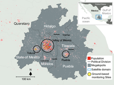
Fig. 1 The blue rectangle in the inset encloses the region (-100ºW to -97ºW, 18ºN to 20ºN) with six states of the Megalopolis of Central Mexico. The red-colored areas correspond to populated urban centers, and the yellow markers represent the ground-based monitoring stations in the Megalopolis with a sufficiency of data (>70%).
2.1 Data validation
2.1.1 Remotely sensed data
Satellite data from the GES-DISC (Goddard Earth Sciences Data and Information Services Center) Interactive Online Visualization ANd aNalysis Infrastructure website (GIOVANNI, 2023) were used to obtain aerosol optical depth (AOD) and other parameters. To ensure data quality, any data sets with a cloud fraction (CF) greater than 70% were excluded (Myhre et al., 2007). Table I overviews the data sets’ parameters, instruments, and spatial and temporal resolutions. AOD daily data were retrieved from both MODIS Aqua (MY) and MODIS Terra (MO) satellites (Sayer et al., 2014) using three algorithms [Deep Blue (DB), Dark Target (DT), and Combined Dark Target and Deep Blue (DTDB)] designed to capture specific features applicable in the study region’s spatial domain. Ground-based remotely sensed AOD measurements from the Aerosol Robotic Network (AERONET; Holben et al., 1998) were used to select the appropriate satellite AOD product. The AOD-AERONET level 3.0 product (AERONET 2021; Smirnov et al., 2000) located at the Universidad Nacional Autonomá de México (National Autonomous University of Mexico) (19.3ºN, -99.18ºW) was used.
Table I Summary of the complete Data Set Used for this study in the spatial domain (-100º to -97ºW, 18º to 20ºN), where D and M mean daily and monthly resolutions, respectively.
| Variable | Product name | Satellite/Instrument | Time res. | Spatial res. |
| AOD-DT | MYD08_D3_v6 | MODIS-Aqua | D | 1º × 1º |
| AOD-DT | MOD08_D3 v6.1 | MODIS-Terra | D | 1º × 1º |
| AOD-DB | MOD08_D3 v6.1 | MODIS-Terra | D | 1º × 1º |
| AOD-DB | MYD08_D3 v6.1 | MODIS-Aqua | D | 1º × 1º |
| AOD-DTDB | MOD08_D3 v6.1 | MODIS-Terra | D | 1º × 1º |
| AOD-DTDB | MYD08_D3 v6.1 | MODIS-Aqua | D | 1º × 1º |
| A-AOD | ----- | AERONET | D | columnar |
| CF | MOD08_D3_v7 | MODIS-Terra | D | 1º × 1º |
| PBLH (m) | M2TMNXFLX | MERRA-2 Model | M | 0.5º × 0.625º |
| NDVI | MOD13C2 v006 | MODIS-Terra | M | 0.05 º |
| RH (%) | AIRS3STD v006 | AIRS | D | 1º × 1º |
| T (ºC) | AIRS3STD v006 | AIRS | D | 1º × 1º |
| SatPM2.5 | M2TMNXAER v5.12.4 | MERRA-2 Model | M | 0.5º × 0.625º |
The AOD-AERONET measurements were taken at 340 nm, 380 nm, 440 nm, 500 nm, 675 nm, 870 nm, and 1020 nm, and interpolation over the wavelength was performed to obtain the corresponding aerosol band AOD-AERONET at 550 nm, the same as AOD from MODIS. Several studies have shown good agreement between satellite and land-retrieved AOD measurements (Bhaskaran et al., 2011; Tripathi et al., 2005). However, Tripathi et al. (2005) found that MODIS overestimates AOD during the Monsoon period, characterized by seasonal wind produced by the displacement of the equatorial belt, resulting in dust transport from other regions. In contrast, MODIS underestimates the AOD observed by AERONET during cold season.
Statistical analysis was performed to examine the data variance and frequency distribution and to determine whether the climatic seasons of the year for the study region influence AOD satellite measurements with MODIS. We assumed that the planetary boundary layer height (PBLH) is a determinant parameter to explain differences between MODIS and AERONET AOD retrieved. Due to the study region having different elevations, the correlation of aerosol particles with AOD varies spatially. PBLH and a proxy of PM2.5 mass concentration were retrieved from the Modern-Era Retrospective analysis for Research and Applications, version 2 (MERRA-2) model (Gelaro et al., 2017). The proxy, SatPM2.5, includes the surface mass concentrations of black carbon, organic carbon, sulfate ion, dust, and sea salt with diameters less than 2.5 μm for calculating SatPM2.5 (Buchard et al., 2016).
2.1.2 Data integration
After selecting the appropriate satellite AOD product (SatAOD) using the process described in the previous subsection, it is necessary to synchronize the data sets of SatAOD, NDVI, PBLH, T, RH, and SatPM2. These data sets come from different instruments and satellites and have varying spatial resolutions. Therefore, a spatial synchronization process is required to compare and use them in a multiple linear regression model. This is achieved through the Inverse Distance Weighting interpolation (IDW) technique using R-code (Gimond, 2022) to interpolate and refine the grids in a mesh (Pebesma, 2004). It should be noted that this technique estimates the new points by taking the average of the nearest neighbors, and contamination at the edge of the spatial domain may occur. Therefore, to avoid this issue, a slightly larger spatial domain (at least two grid cells) than the one shown in the inset in Figure 1 is considered.
The refined raster layers obtained (5.5 km × 5.5 km) are clipped according to the extent shown in Figure 1, and verification is done to ensure that the data distribution has not been altered. It is also essential to consider the scale, as previous research has shown that the scale is crucial in the bias of regression model outputs (Paciorek, 2010). Additionally, studies have reported that the correlation between AOD and PM2.5 decreases when the AOD resolution is reduced (Chudnovsky et al., 2013). Finally, the monthly mean average of variables is calculated to complete the data integration process.
2.2 Data correlation
To ensure that the model has desirable features such as low or no correlation among independent variables but significant influence on the dependent variable (PM2.5), it is crucial to investigate the possible correlation between the independent and dependent variables before using variable data to build the model. This investigation can be carried out using the Raster package in R (Raster Package, 2023).
Local correlation is recorded for the central grid, and the operation is repeated throughout the entire domain in the raster. To use the function in two rasters simultaneously, an intermediate step involves defining a third raster that records the positions of the values of each grid, listing them from 1 to the total number of grids. The focal function then extracts the positions for which values from the two rasters are obtained.
This technique helps to investigate the spatial correlation between the independent variables (NDVI, T, RH, PBLH, AOD) and the dependent variable (PM2.5) on a monthly or quarterly season basis (MAM, JJA, SON, and DJF). It allows for identifying differences in areas of the study region due to various factors such as human activity, meteorology, soil types, and characteristics of each sub-region.
Finally, the correlation between the two variables in each grid is shown on a map, highlighting regions where the correlation between the variables is negative (-1), null, or positive (+1). This map can help to refine the model further, ensuring that it meets the desirable features required for accurate predictions of PM2.5 levels.
2.3 A Model to estimate PM 2.5 concentration
In summary, the study incorporates six AOD products derived from Aqua and Terra satellites, processed with three different algorithms, to find the most suitable AOD variable that explains SatPM2.5 concentrations. The data are integrated and synchronized spatially and temporally before using them in a linear regression model that includes satellite-retrieved variables (SatAOD, NDVI, PBLH, RH, and T) in each grid and month of the simulation domain. Before model construction, spatial and temporal correlation analyses are conducted among the variables. The proposed linear regression model is expressed as follows:
The multiple linear regression model’s parameters (α0, α1, …, α5) are adjusted to obtain the best fit with the observed data at monitoring sites (TeoPM2.5). The process begins by considering all variables as predictors and selecting the best ones using the Akaike Information Criterion (AIC). AIC is a metric used to compare the fit of multiple regression models, with a smaller AIC indicating a better fit (Sakamoto et al., 1986). The AIC penalizes models with excessive independent variables based on their ability to explain the dependent variable. It yields the lowest score for a model with minimal loss of information or the highest predictive power while minimizing the number of predictor variables. Various R-Studio libraries (stats v3.6.2, olsrr 0.5.3) are utilized to perform the analysis. The “confinity” function in R (stats v3.6.2, n.d.) estimates the confidence intervals for the parameters in the fitted regression model.
2.3.1 PM 2.5 Ground-based measurements
To validate the performance of the regression model, ground-based PM2.5 concentrations for the study region were obtained from multiple sources, including the National Air Quality Information System (SINAICA, 2021) and the Mexico City’s automatic air quality monitoring network (Red Automática de Monitoreo Atmosférico, or RAMA) (RAMA-CDMX, 2021; RAMA-EdoMex, 2021). 13 monitoring stations with a sufficiency rate > 70% located in Mexico City and the State of Mexico were selected. Hourly PM2.5 concentration data from these stations were carefully verified, and suspected outliers were removed. These ground-based PM2.5 data were then compared with the PM2.5 values estimated by the regression model (TeoPM2.5) to assess the model’s efficiency.
3. Results
3.1 Satellite AOD validation
The correlation analysis between the six AOD products and SatPM2.5 revealed a high R2 value ranging between 0.73 and 0.76, except for AOD from MODIS Aqua DTDB, which had an R2 of 0.59. Among the six products, AOD from MODIS Terra DT showed the highest correlation (R2=0.76), indicating its suitability for the linear regression model. In addition, the AOD grids (3×3) generated by each algorithm and platform were compared with the AERONET network’s point data to gain further insights into AOD selection. Figure 2 shows the monthly correlation results of AOD from MODIS-Terra (MO) and MODIS-Aqua (MY) for each algorithm: DT, DB, DTDB, and AOD from AERONET.
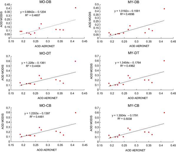
Fig. 2 Monthly AOD correlation between AERONET and MODIS Aqua (MY) and MODIS Terra (MO) products (DB, DT, and DTDB) for the 2012 year.
Although the Aqua and Terra algorithms used for processing satellite data are similar, there is a better correlation coefficient with Aqua than with Terra. The dry-hot season, from March to May, is characterized by higher AOD values, especially in May, as seen in Figure 3.
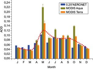
Fig. 3 Comparison of AERONET monthly AOD averages and MODIS Terra and Aqua (DB) monthly and spatial (0.25) AOD averages in 2012. The red-dotted line represents the monthly mean trend.
In May, the AOD data from MODIS Terra and Aqua satellites, as well as the rescaled (0.25) AOD-AERONET data, showed unexpectedly high values compared to the expected trend. This indicates that the satellite data may capture particles in the upper atmosphere that cannot be detected with the same precision by AERONET measurements from the surface. The DB product used for processing satellite data does not differentiate between fine and coarse mode aerosols, which could explain the lack of differentiation between dry-hot season (MAM) and cold quarter (DJF). However, the presence of coarse particles from wildfires during the dry-hot season (MAM) suggests otherwise. In October, there were discrepancies between the MODIS and AERONET data trends, with (0.25) AOD-AERONET slightly below the expected trend and AOD MODIS data above it. This could be attributed to the challenges of remote sensing measurements during the rainy season (June-August).
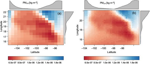
To refine the grids of the mesh, various interpolation algorithms were applied using the “gstat” package in R (Gimond, 2022). The Inverse Distance Weighting (IDW) method was chosen to estimate new points, considering the nearest neighbors’ average value (nmax = 5). This method assigns greater weight to the closest points, thus providing a more precise estimate. Figure 4 illustrates the data integration step, displaying the PM2.5 data obtained from remote sensing (Sat-PM2.5) before and after the mesh refinement for January 2012. The gray-colored plots reveal that the spatial distribution remained unchanged after synchronization. To avoid data contamination at the region’s edge, the refined mesh (Figure 4b) was cropped according to the spatial domain extent, which was larger than the region of interest in this study.
3.2 Correlation among variables
To ensure accurate predictions, a linear regression model must have independent variables that are not highly correlated with each other but rather have some correlation with the dependent variable (PM2.5). Figure 5 shows the correlation among satellite-retrieved variables during the March-May 2012 quarter. During the dry-hot season, from March to May, the dependence of AOD on temperature increases, with values of +0.4, +0.5, and +0.7, respectively. Poor green vegetation profiles and wildfires, including those set for agricultural purposes in the Megalopolis of Central Mexico, can contribute to the resuspension of particles and the resulting increase in AOD. Likewise, during the dry-hot season, the PBLH has a negative correlation with PM2.5 that decreases from -0.4 (march), -0.3 (april) to -0.2 (may). This means as temperature increases, the height of PBLH also increases, leading to a decrease in the correlation between PBLH and PM2.5. Similarly, the correlation between PBLH and AOD during the dry-hot season (MAM) ranges between -0.4 to -0.6, suggesting that aerosols’ cooling effects in the lower PBLH can suppress the development of PBLH, as reported by Zhang et al. (2022).
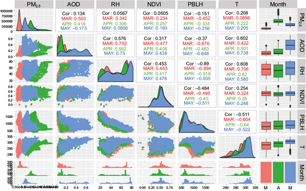
Fig. 5 Correlation of satellite-retrieved variables for dry-hot season months (March, April, and May) in 2012 in the Megalopolis of Central Mexico.
Figures 6 and 7 illustrate the monthly spatial correlation between Sat-PM2.5 and AOD and Sat-PM2.5 and PBLH5, respectively, within the study region outlined by a black rectangle. The warm colors (red) indicate a positive correlation (+1), while the cool colors (blue) indicate a negative correlation (-1). During the dry-cold season Sat-PM2.5 and AOD, from Figure 6, exhibit a high positive correlation in the east, north, and northeast regions of the spatial domain. But, the center, south, and southwest areas present a high negative correlation. The difference in the correlation between these two regions is likely explained by the significant elevation gradient, which implies substantial differences in vegetation, soil type, and meteorology.

Fig. 6 Monthly mean spatial correlation between Sat-PM2.5 and AOD in the study region (-100º to -97ºW, 18º to 20ºN) enclosed by the black rectangle.
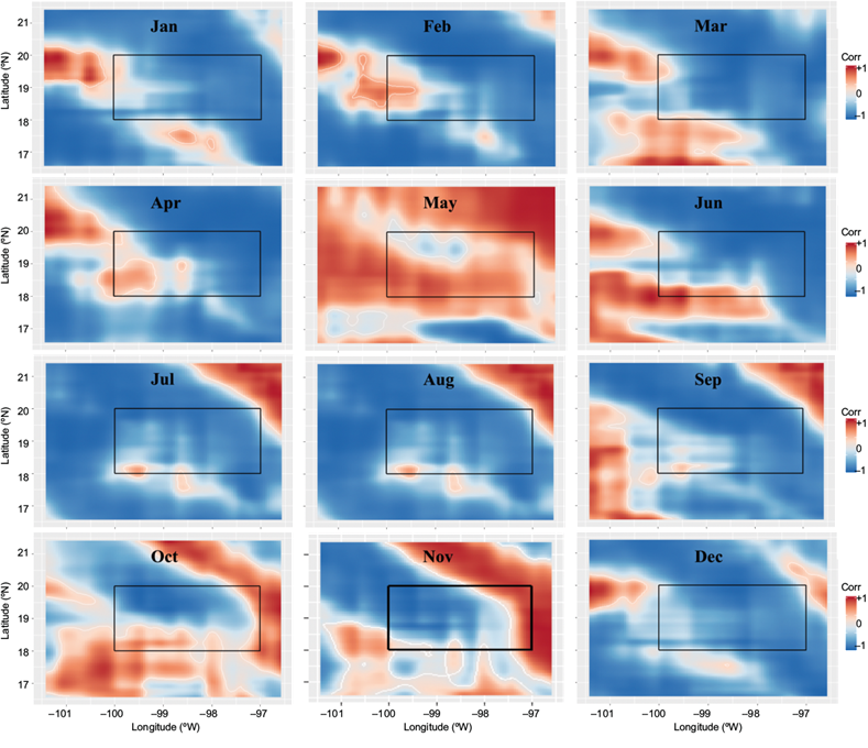
Fig. 7 Monthly mean spatial correlation between Sat-PM2.5 and PBLH in the study region (-100º to -97ºW, 18º to 20ºN) enclosed by the black rectangle.
The spatial correlation of Sat-PM2.5 and PBLH presented in Figure 7, shows negative values during the cold season (DJF), coinciding with the lowest values of the PBLH and high episodes of particle matter, which are observed systematically in México City during the winter. In the following months, the negative spatial correlation is observed up to March, but in April and May, the spatial correlation changes to positive, which certainly means that if PBLH increases, then PM2.5 also does. This outcome underscores the significance of emissions transport from areas outside the megalopolis. It helps to clarify the persistently high ozone levels or particles observed systematically despite the local mitigation strategies employed in Mexico City during the dry hot season (MAM).
3.3 Ground-based PM 2.5 Analysis
Figure 8 presents the boxplots of annual PM2.5 concentrations measured at selected monitoring sites in Mexico City during 2012. The boxplot displays the median, first, and third quartile values, while the suspected outliers are indicated with red circles. These outliers are data points that lie beyond 1.5 times the interquartile range (IQR) from the upper and lower quartiles. After removing the outliers, the lower and upper fences of the box represent the minimum and maximum values, respectively.
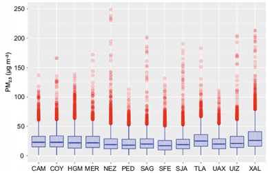
Fig. 8 Annual PM2.5 concentrations on ground-based monitoring sites in Mexico City. The red circles represent the extreme values (suspected outliers).
Figure 9 shows the hourly, daily, and monthly average concentrations of PM2.5 in Mexico City. Figure 9a shows that the hourly analysis by day of the week reveals two peaks, one before noon (11 a.m.) and another in the late afternoon (7 p.m.), consistent throughout the week. However, two monitoring sites in the northern part of the city, XAL and SAG, exhibit earlier peak concentrations (around 40 minutes earlier) than other sites, with XAL having the highest PM2.5 levels. Figure 9b (lower-left corner) summarizes the hourly averages by day of the week and shows two distinct peaks in PM2.5 concentrations throughout the day. Figure 9d (lower-right corner) shows the averages by day of the week, demonstrating that PM2.5 accumulates during the week, with the highest levels observed on Friday or Saturday. After reductions in emissions from vehicles and industries during the weekend, the lowest levels are observed on Monday. The monthly averages in Figure 9c (lower-middle part) exhibit two peaks, one in May and another during the cold season (DEF). The latter corresponds to the maximum PM2.5 levels Fontes et al. (2017) observed, as thermal inversion traps pollutants. For a detailed discussion of the observed peaks and the main sources of PM2.5, see Mora et al. (2017).
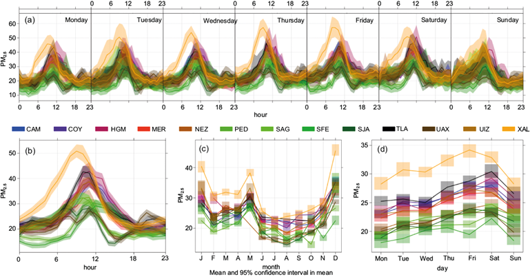
Fig. 9 The (a) hourly by day of the week PM2.5, (b) hourly, (c) monthly, and (d) day of the week average PM2.5 concentrations at ground-based monitoring sites in Mexico City in 2012.
Figure 10 highlights specific characteristics of the quarterly hourly averages of PM2.5 data. The highest concentrations of particles are observed during the dry-hot season (March to May) and the cold quarter (DEF). Precipitation during the rainy season (June-August) contributes to removing PM2.5. However, two peaks are still observed yearly in PM2.5 levels despite the removal effect. The first peak occurs during the dry-hot season (MAM) when intense wildfires and maximum PBLH (as shown in Figure 11b) facilitate the exchange of air masses from other territories. In contrast, another peak is observed during the cold season (DEF), and the height of the PBLH reaches a minimum, indicating that the study area is relatively isolated from the neighboring regions. This isolation results in lower dilution of pollutants and an increase in PM2.5.

Fig. 10 Hourly averages by quarter (March-May, June-August, September-November, December-February) of PM2.5 concentrations at monitoring sites in Mexico City in 2012.
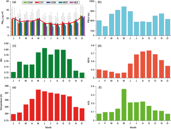
In Figure 11, monthly means of remotely sensed data, including PBLH, RH, T, AOD, and NDVI, are presented with the corresponding ground-based PM2.5 measurments. Notably, PM2.5 concentrations from MERRA-2 and ground-based sites exhibit the same qualitative trend. However, PM2.5 levels from ground-based sites show a different trend than AOD during the cold season (DJF).
3.4 Linear regression model fit
Table II presents the monthly correlation coefficients for each variable from the multiple linear regression model (TEO PM2.5). The alpha parameters have standard errors ranging from 1e-13 to 1e-11 and p-values less than 1e-16, indicating high statistical significance.
Table II Multiple linear model (TeoPM2.5) correlation coefficients.
| α0 | α1 AOD | α2 NDVI | α3 PBHL | α4 RH | α T | |
| January | 2.86e-10 | 2.00e-09 | -8.21e-11 | -1.90e-13 | 5.65e-12 | -1.49e-11 |
| February | 1.18e-10 | 5.20e-10 | 1.05e-10 | -1.33e-13 | 7.48e-12 | -1.30e-11 |
| March | 7.56e-10 | 1.81e-09 | 1.78e-11 | 1.08e-14 | 9.09e-13 | -1.68e-11 |
| April | 2.27e-10 | 1.33e-09 | 2.85e-10 | 3.59e-13 | 1.06e-11 | -5.26e-12 |
| May | 8.84e-10 | -1.81e-10 | 1.09e-11 | 1.44e-14 | -2.26e-12 | 3.31e-12 |
| June | 2.23e-09 | 4.82e-09 | -1.99e-09 | -8.71e-13 | -1.83e-11 | 3.56e-11 |
| July | 2.54e-09 | 2.23e-08 | -8.42e-09 | -3.57e-12 | 1.16e-10 | 6.92e-11 |
| August | 7.08e-09 | 6.02e-09 | -2.03e-09 | -5.19e-12 | -2.01e-11 | 6.03e-11 |
| September | 7.97e-10 | 1.57e-09 | -1.12e-09 | -4.23e-13 | 6.36e-12 | 4.24e-12 |
| October | 2.19e-10 | 1.33e-10 | -3.73e-11 | 4.07e-14 | -4.24e-12 | 9.32e-12 |
| November | -2.12e-10 | 8.34e-10 | -7.57e-11 | 1.67e-13 | 1.00e-11 | -1.40e-11 |
| December | 1.14e-09 | 3.10e-09 | -1.81e-10 | -8.18e-13 | 1.20e-12 | -1.76e-11 |
Using the multiple linear regression model coefficients, PM2.5 levels were estimated for each grid in the study area. The model, which incorporated all variables as predictors, exhibited a high R2 value of 0.7501, indicating that it can account for 75.01% of the observed variability in life expectancy. The p-value of the model was significant (3.787e-10), further supporting its validity. The spatial distribution of calculated PM2.5 concentrations is displayed in Figure 12. Monthly trends in the estimated PM2.5 values show good agreement with those obtained from the MERRA-2 model. Comparison of the estimated monthly PM2.5 concentrations with corresponding monitoring sites in Mexico City resulted in a 0.6-0.8 RMSE and a standard deviation of 0.01-0.5 µg.
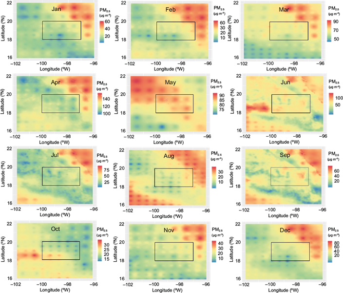
Fig. 12 Monthly mean PM2.5 concentrations calculated from the multiple linear regression model (TeoPM2.5) for the spatial domain in this study (enclosed by the black rectangle).
The most significant discrepancies between estimated and observed PM2.5 concentrations occurred during the rainy season (June to August) when aerosol retrievals from satellites were challenging. Conversely, the dry-hot season (MAM) provided the most favorable conditions for estimating PM2.5 concentrations with the model. Estimated PM2.5 values in Puebla exhibited lower confidence (0.4-0.6 RMSE) than those in Mexico City.
Figure 13 depicts the monthly PM2.5 concentrations calculated for each grid cell (TEO PM2.5) compared to the corresponding ground-based monitoring sites, Xalostoc (XAL) in Mexico City and Ninfas (NIN) in Puebla, for the base year 2012. In general, the modeled PM2.5 concentrations show a similar trend to the ground-based monitoring sites in both cities, with peaks occurring during the dry-hot season (MAM) and winter. However, the model results overestimate the ground-based PM2.5 concentrations during the dry-hot season (MAM) and in August.
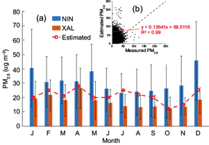
Fig. 13 Monthly mean PM2.5 concentrations in 2012 from multiple linear regression model (TeoPM2.5, estimated; red-dotted line) and ground-based monitoring measurements in (a) Xalostoc (XAL) in Mexico City (19.526ºN, -99.082ºW) and Ninfas (NIN) in Puebla (19.043ºN, -98.214ºW). The inset (b) summarizes the correlation between estimated PM2.5 concentrations (TeoPM2.5) and all the monitoring sites in Mexico City, the State of Mexico, and Puebla.
4. Conclusions
The study utilized spatially and temporally synchronized satellite data to investigate the relationship between several variables and environmental PM2.5 concentrations. It was discovered that the correlation between AOD and PM2.5 is influenced by RH, PBLH, and T. Based on AERONET calibration, using the AOD DB product for studying PM2.5 in the Megalopolis of Central Mexico is recommended. PBLH is a crucial parameter in explaining the differences between MODIS and AERONET AOD retrieval. The spatial correlation analysis revealed a significant change in the relationship between PBLH and AOD towards the end of the dry-hot season (MAM), highlighting the importance of emissions transport from regions beyond the MCM. This information provides insights into potential mechanisms that could explain persistently high ozone levels or particulate concentrations despite local mitigation strategies during the dry-hot season (MAM).
The study developed a multiple linear regression model to estimate environmental PM2.5 levels. The research hypothesis that AOD data (MODIS) can estimate PM2.5 concentrations in the megalopolis of Mexico was confirmed. However, caution must be exercised in interpreting the model results since the analysis previous to the model revealed significant changes in the correlations of AOD, T, RH, and PBLH during each of the four climatic seasons. The model produced satisfactory results during the dry-hot season (MAM) but failed during the rainy season (June-August). Finally, the concentrations of PM2.5 in the study area are influenced by fire emissions, and incorporating fire data as an additional variable could enhance the model’s performance during this time of year (Jaffe et al., 2008; Vega et al., 2021).

