1. Introduction

Climate is changing and the main indicator is above surface ambient temperature, as detailed in the 2013 Intergovernmental Panel on Climate Change report (^{IPCC, 2013}). There are different sources that demonstrate that the mean ambient temperature for the Northern Hemisphere (^{Jones and Mann, 2004}; ^{Piacentini and Mujumdar, 2009}) and for the whole world (^{Nazarenko et al., 2015}; ^{Weart, 2018}) has been increasing significantly in the last decades. Evidence of this increase may be seen in the effect that the above surface air temperature has had on the sub-surface temperature for the first hundred meters (^{Jessop, 1990}; ^{Weart, 2008}).

When Earth’s atmosphere experiences a temperature change, the soil in contact with the atmosphere will feel this change. Then, the Earth’s surface thermal disturbance propagates into the subsurface by heat conduction through the soil. This thermal disturbance at the Earth’s surface propagates downward as a type of thermal wave (^{Carslaw and Jaeger, 1959}). According to the theory of heat conduction, temperature diminishes its amplitude exponentially with depth and this attenuation is frequency-dependent. Lower-frequency waves propagate to greater depths than higher-frequency waves (Carslaw and Jaeger, 1959). High-frequency (diurnal and annual) variations in ground surface temperature vanish in the first meters (up to around 20 m) beneath the surface, and low-frequency variations in ground surface temperature vanish in the first hundred meters (^{Pollack and Huang, 2000}). Changes in the ground heat flow introduce a curvature to the linear temperature steady-state thermal regime behavior. Furthermore, in this long-term trend, a variety of processes at or near the ground surface may perturb downward propagating subsurface temperature and they may mask the magnitude of temperature change attributed to climatic change. Those processes are changes in snow cover (^{Groisman et al., 1994}), changes in land use and land cover (^{Lewis, 1998}; ^{Skinner and Majorowicz, 1999}), and urbanization (^{Kalnay and Cai, 2003}). Therefore, to attribute at least partially the subsurface transient temperature to climate change (or global warming), it is necessary to rule out non-global-change processes in the present heat transfer model calculation, in the period of time under study (1970-2200) for Kapuskasing, Canada

The aims of this study are: (1) to identify, from model calculation considering the Fourier heat transfer equation, the time-varying subsurface temperature from the boundary condition on the Earth’s surface to the inner part of the soil at the Kapuskasing site (49.41-82.47º), Canada; (2) to make a modeling of the one-dimensional heat conduction into the subsurface using the time-varying boundary condition identified for this site, by a forward modeling approach, fitting the temperature measured underground at the year 1970; (3) to estimate the diffusivity of the soil; (4) to quantify the behavior of the downward propagating thermal signal (temperature and heat flux) for the year 1970, and (5) the future behavior (assumed to be due only to global warming) of the sub-surface temperature considering the four ^{IPCC (2013)} Representative Concentration Pathway scenarios: RCP2.6, RCP4.5, RCP6 and RCP8.5. These scenarios correspond to different trajectories of greenhouse gases concentrations, describing possible climates in the future, where the numbers are values of radiative forcing, which is a measure (in W m^-2) of the net atmospheric radiation energy balance at the end of the present century (2100). RCP2.6 is associated with a relatively low world emission of greenhouse gases (with humanity making a significant effort for the mitigation of climate change), RCP4.5 to intermediate emissions, RCP6 to medium-high emissions and RCP8.5 to high emissions. The radiative forcing associated with the RCP2.6 scenario (the most optimistic one) will increase with time up to a maximum value of about 3 W m^-2 in the decade of 2040, followed by a continuous decline in the rest of the present century, crossing the years 2100 and 2200 with values of 2.6 and 2 W m^-2, respectively. The radiative forcings associated with RCP4.5 and RCP6 increase continuously and stabilize at around 2150, at values of 4.5 and 6 W m^-2, respectively. The RCP8.5 scenario (the most pessimistic radiative forcing) also increases continuously, having values of 8.5 and 12 W m^-2 by 2100 and 2200, respectively (^{IPCC, 2013}).

2. Materials and methods

In order to analyze the temperature-depth profiles, the solution to the heat conduction equation of a continuous medium given by ^{Carslaw and Jaeger (1959)} is considered;

where ρ is the density of the medium, c _p the specific heat at constant pressure, λ the thermal conductivity, ∇ the vector differential operator, and Q´S the heat production rate per unit volume.

The assumptions of our model are: (1) the heat production can be neglected Q´S≈0 for the borehole analyzed in this study because the depth of the borehole is only a few hundred meters; (2) the advection of heat is neglected (v.∇T = 0); (3) the soil (near the surface) is a near homogeneous semi-infinite half space, which means that topographic and groundwater effects (^{Blackwell et al., 1980}; ^{Bodri and Cemák, 2005}; ^{Bense and Beltrami, 2007}), which could perturb heat transfer, are neglected, and (4) the lithologic sequences in the site have uniform thermal properties, thus the conductivity and diffusivity are considered constant with respect to depth.

With these assumed conditions, the temperature at a given depth z is determined by the superposition of both the steady-state solution and the time dependent transient perturbation:

where T _ss (z) is the steady-state solution and T _t (z, t) is the transient perturbation solution:

where T ₀ is the mean long-term surface temperature and Γ ₀ is the thermal gradient of the steady-state.

The transient subsurface temperature component, with a given assumed air temperature boundary condition, is calculated from the following simplified version of the one-dimensional heat conduction equation (Eq. [1]):

where k = λ/(ρc _P ) is the thermal diffusivity.

Following Marechal and Beltrami (1992), the solution to Eq. (4) in the period 1880-1940 can be expressed as the following sum of M terms:

where T _m is the surface temperature mean value at each time interval (t _m , t _m-1 ) and erfc the complementary error function erfc(x) = 1 - erf(x) = 1 - 2/ π∫ ₀ ^x exp(-u ² )du. After several tests employing the forward model, a value of M =12 was fixed (corresponding to a time interval of 5 years).

Figure 1 describes the subsurface temperature as a function of depth, for Kapuskasing, Canada as given by ^{Cermák (1971)}, showing a concave behavior towards higher temperatures in the year of measurements (1970), with respect to a steady state situation implying no perturbation in the year 1880. This is the year of the onset of the subsurface temperature change within the time interval 1850-1900 determined by ^{Beltrami et al. (2003)} for Kapuskasing, southeast Canada. It should be noted that these authors show similar behaviors as those presented in Figure 1 for other sites of Canada, confirming the significant change in sub-surface temperature near surface partially due to climate change. In order to obtain the best adjustment to the measured data displayed in Figure 1, the ^{Cermak (1971)} temperature boundary condition was considered. As another confirmation of this behavior, ^{Hamza and Vieira (2011)} presented the same concave subsurface temperature behavior for the Southern Hemisphere site of Juazeiro, Brazil, with no convex subsurface temperature variation with depth (which would indicate a cooling effect).

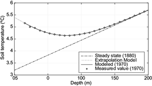
Fig. 1 Time evolution of the subsurface temperature at the Kapuskasing site in the Northern Hemisphere. Measured data for this site are represented as circles. Model calculations curves are obtained from the solution to the heat conduction differential equation for a given time. The dotted line in the soil depths near surface is an extrapolation of the model calculation curves. The straight line corresponds to the asymptotic behavior in the steady state. 

Following ^{Cermak (1971)} and ^{Beltrami et al. (2003)}, in this work the steady state behavior is assumed to start in the year 1880. We describe the steady-state solution for Kapuskasing as T _ss (z) = 3.2 + 0.0125. z.

Traditional analysis of temperature depth profiles to obtain ground thermal information is based on the forward model approach to fit the measured data (e.g., ^{Birch, 1948}; ^{Beck and Judge, 1969}; ^{Cermák, 1971}; ^{Cermák and Jessop, 1971}; ^{Sass et al., 1971}; ^{Beck, 1977}; ^{Vasseur et. al., 1983}; ^{Clauser, 1984}; ^{Lindqvist, 1984}; ^{Lachenbrunch and Marshall, 1986}; ^{Wang et al., 1986}). To run a forward model approach, we need to identify the (temperature) time-dependent boundary condition acting on the surface, during the period between the year of relative steady-state regime to the year of measured temperature values.

In the present work and for the studied period, the change in surface temperature is partially attributed to climate change, without considering other processes. This assumption has also been suggested by other authors, like those detailed in the previous paragraph and by ^{Hamza and Vieira (2011)} for the Southern Hemisphere.

From the main assumption of the forward model approach that the lowermost part of the borehole data is absent of transient temperature behavior (as is evident from the almost linear behavior for depths higher than about 170 m [see Fig. 1]), it is possible to extrapolate to lower depths this linear behavior, obtaining in this way the value of the surface temperature at the proposed year (1880), as was also determined by ^{Beltrami et al (2003)}.

The quality of the model calculation results of the subsurface temperature as a function of depth, represented by Eq. (5), was analyzed by comparing these results with the measured data in Kapuskasing, Canada (^{Cermák, 1971}). Applying the least square method, the thermal diffusivity (k) introduced in Eq. (4) was adjusted, giving rise to the following value and corresponding error: k = (1.022 ± 0.015).10^-6 m² s^-1, with a percentage error of only 1.5 %.

3. Results of the past behavior of subsurface temperature induced by climate change

In order to make a model calculation for the borehole temperatures and for an extrapolation to the future for Kapuskasing, Canada, in the Northern Hemisphere, the annual mean temperature boundary condition at the surface as a function of time was considered (^{Extreme Weather Watch, 2021}). These data were treated with a minimum square approximation, obtaining linear increase with a slope of 0.48 ± 0.11 ºC per decade from 1970 to 2010.

Following ^{Baker and Ruschy (1993)} and ^{Putman and Chapman (1996)}, a long-term coupling between ground surface temperature and surface air temperature is assumed. With respect to the effects that can be responsible for the modification of the subsurface temperature as a function of time, besides climate change, perturbations due to urbanization processes, solar radiation modifications (which can produce changes in evapotranspiration), and snow cover, can also contribute to changes in the subsurface temperature.

Considering the boundary conditions mentioned and using the (approximate) solution to the differential heat equation that describes the heat conduction through the soil given in Eq. (5), Figure 1 presents model calculation results of the time evolution of the subsurface temperature for Kapuskasing from the depth of the first measured point to greater depths. An extrapolation is made from this first measured point to the surface, to obtain the temperature at z = 0 m. The measured data of ^{Cermak (1971)} for Kapuskasing are also detailed in the same figure.

Considering the value of conductivity as λ = 2.64 W mK^-1 (^{Jessop et al., 1984}) for Kapuskasing, the heat flow is also calculated using the following (well known) formula: J = λ × dt dz ^-1 , as given in Figure 2. The heat flow value for Kapuskasing at 200 m depth is -0.033 W m^-2, which is coherent with that obtained by ^{Chouinard and Mareschal (2009)} in a near site.

Fig. 2 Time evolution of the subsurface temperature at Kapuskasing in the Northern Hemisphere. Measured data for this site are represented as circles. Model calculation curves are obtained from the solution to the heat conduction differential equation for a given time. The dotted line in the soil depths near the surface is an extrapolation of the model calculation curves. The straight line corresponds to the asymptotic behavior in the steady state. 

From the model calculation results (obtained for the years 1880 and 1970) for sub-surface temperature, the following characteristic values were determined (see Table I): (a) depth z _max,t , where the surface perturbations had reached practically its final propagation at time t when the measurements were performed (through the condition of a 0.01 ºC difference with respect to the asymptotic linear behavior); (b) the depth z _t *, where the subsurface temperature changes its slope from negative to positive variation in a particular year; c) the temperature gradient γ _0,t = ∂T/∂t _z=0,t at surface for the year 1970; (d) the thermal gradient at steady state Γ _0,1880 in the starting year (1880); (e) the temperature differences between 1970 in Kapuskasing and the initial year 1880, extrapolated to surface (∆T _z=0 ) and z=20 m (∆T _z=20m ) (this last value corresponds to the depth at which the hourly and daily surface perturbation practically disappears), and (f) the heat flow at surface to the inner part of the soil, attributed to climate change.

3.1 Time evolution of different future scenarios for sub-surface temperature

Figure 3 presents the time evolution of sub-surface temperature at Kapuskasing, Canada, subject to surface temperature boundary conditions as described in the text and an RCP8.5 future scenario, for the years 1880 (straight line), 1970 (solid curve almost coinciding with the measured points), 1990-2190 (one solid curve every 20 years corresponding to surface temperature as boundary conditions of increasing values), and 2200. The large impact attributed to climate change near surface is evident since the temperature boundary condition on surface has the largest expected difference of all scenarios (with a value of 8.3 ºC, see Table II) in the 1970-2200 period. At the largest analyzed depth (z = 200 m), the perturbation due to the external surface driver is rather small (0.7 ºC).

Fig. 3 Sub-surface temperature as a function of the depth for Kapuskasing, Canada considering the RCP8.5 future Representative Concentration Pathway (RCP) scenario (IPCC, 2013). The straight line describes the linear thermal steady state behavior in the year 1880. Measured data for 1970 (^{Cermák, 1971}) are represented by circles. The sub-surface temperature distribution determined every 20 years (from 1990 to 2190, including also 2200) is detailed in solid lines. 

Table II Changes in temperature from 1970 to 2200 for Kapuskasing, Canada for a given depth and for a given IPCC (2013) scenario. 

	Kapuskasing
RCP	2.6	4.5	6	8.5
ΔT (z = 0 m)	2.7 ºC	3 ºC	5 ºC	8.3 ºC
ΔT (z = 100 m)	1.7 ºC	1.8 ºC	2.4 ºC	2.8 ºC
ΔT (z = 200 m)	0.6 ºC	0.6 ºC	0.7 ºC	0.7 ºC

RCP: Representative Concentration Pathway (IPCC, 2013).

Figures 4 and 5 show similar behaviors as Figure 3, but for the RCP6 and RCP4.5 future scenarios, respectively. In these cases, the temperature difference at ground in the period 1880-2200 (and also at all depths) shows lower values than those of the RCP8.5 scenario, as given in Table II.

Fig. 4 As in Figure 3, but for the RCP6 future scenario. 

Fig. 5 As in Figure 3, but for the RCP4.5 future scenario. 

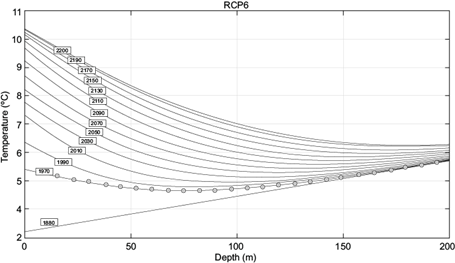
Figure 6 has a similar behavior as Figure 3 for the RCP2.6 future scenario, except for the period 2090-2190 (one solid broken curve every 20 years) and the year 2200. In these cases, a particular behavior can be observed, since near surface the evolution of sub-surface temperature does not follow the constant increase at all depths, as in the other three scenarios. This effect is because surface temperature verifies boundary (at surface) conditions of decreasing values after passing a maximum around year 2070.

Fig. 6 As in Figure 3, but for the RCP2.6 future scenario. Dashed lines correspond to curves where the change in near-ground surface temperature is decreasing for the corresponding year, with respect to the maximum attained value at surface. 

Table II details temperature differences at surface and 100 and 200-m depths for Kapuskasing and for the four IPCC (2013) scenarios. The differences were calculated for the period of available data (1970) and the end of the next (2200). Maximum differences are obtained at ground surface, ranging from 2.7 ºC for the low emission RCP2.6 scenario to 8.3 ºC for the high emission scenario (RCP8.5). At the highest depth (200 m), the surface temperature perturbation partially attributed to climate change is 0.6 ºC for RCP2.6 and RCP4.5 scenarios, and 0.7 ºC for RCP6 and RCP8.5 scenarios.

Table III presents a comparison of temperature changes at surface, mainly in the present (1980-2080) and in the next (2080-2180) centuries, and for each IPCC scenario (IPCC, 2013). It can be seen that most of the changes in temperature occurred during the first 100 years in all scenarios except for the extreme one (RCP8.5).

Table III Temperature changes at surface at the Kapuskasing site, Canada, for a 100-year interval, in (mainly) the period 1880-1980, the present century (1980-2080), and the next century (2080-2180), for each IPCC (2013) scenario. 

RCP8.5
1880-1980	2.7 ºC
1980-2080	4 ºC
2080-2180	3.5 ºC
RCP6
1880-1980	2.7 ºC
1980-2080	3.1 ºC
2080-2180	1.3 ºC
RCP4.5
1880-1980	2.6 ºC
1980-2080	2.3 ºC
2080-2180	0.2 ºC
RCP2.6
1880-1980	2.6 ºC
1980-2080	2.2 ºC
2080-2180	-0.2 ºC

RCP: Representative Concentration Pathway (IPCC, 2013).

4. Impact of the variation in soil temperature due to climate change in near-surface geothermal energy

One of the significant uses of geothermal energy (the energy extracted from the soil) is the production of energy from the difference between ambient air temperature and sub-surface temperature. With the help of underground tubes placed between some meters to dozens of meters of depth, it is possible to obtain temperature differences normally in the range of 5-10 ºC, increasing the winter ambient temperatures and decreasing the summer ones. Another application is in a geothermal heat pump, equipment that extracts energy from the ground from depths of about 300 m, normally for climatization purposes (^{Lund, 2018}).

From the results presented in Figure 3 for Kapuskasing in the Northern Hemisphere, it is possible to foresee the future impact of global warming in these low and medium-depth geothermal systems:

5. Conclusions

From the results obtained in the present work, the following conclusions can be derived: