


 nueva página del texto (beta)
 Inglés (pdf)
 Artículo en XML
 Referencias del artículo
 Enviar artículo por email
 Citado por SciELO
  Similares en
SciELO
Similares en
SciELO 
 Permalink
1. Introduction
During summertime in South America, the South Atlantic Convergence Zone (SACZ) has a major influence on the precipitation regime. The SACZ is responsible for about 25% of the rainfall volume across southeastern Brazil between the months of October to April (Nielsen et al., 2019), which, along with the convection in the rainforests of the Amazon River basin, are important factors of the South American Monsoon System (SAMS) during its active phase (Carvalho et al., 2004).
Some typical characteristics of the SACZ are the flow in around 200 hPa, the Bolivian High (BH), and an upper-troposphere cyclonic vortex over the northeast of Brazil to the east of the BH, whose formation is dynamically linked to the presence of the BH and to the convection associated with summertime heating in the Amazonian region. Near the surface, there is the moisture convergence in the NW-SE direction, resulting in horizontal wind divergence in high atmospheric levels and (Quadro, 1999).
The SACZ can then be identified as a region of moisture convergence from the low levels to the mid-troposphere, with a convective cloud cover oriented from northeast to southeast that persists for at least four consecutive days and extends from the southern Amazon to the southwest Atlantic Ocean (Kodama, 1992; Quadro, 1999; Carvalho et al., 2004).
The position of the SACZ is a consequence of a deep convection of the Amazon Basin that makes the development of a SACZ around 12 to 18 h after a peak of the Amazon convection, highlighting the importance of the moisture flux from the Amazon, although extratropical cyclones and fronts are essential to maintain the SACZ dynamics (Figueroa et al., 1995; Lenters and Cook, 1995; Ambrizzi and Ferraz, 2015).
There is a seesaw pattern attributed to the dipole within the precipitation in the SACZ areas (Carvalho et al., 2004). The SACZ plays a fundamental role in the hydrological cycle of the regions affected by the SACZ variability in the continent and its compensation mechanism over northeast Argentina, Uruguay and southern Brazil (Gandu and Silva, 1998; Muza et al., 2009).
The motivation for this work lies in the importance of identifying and anticipating with better accuracy the occurrence of intense and/or persistent rainfall since several social and economic factors are associated with the intense rainfall typical of the SACZ. Investing in meteorological studies that can help in the prevention or mitigation of natural disasters can lead to action planning with proper supporting measures to alert people who live in hazardous areas (Vera et al., 2006; Nielsen et al., 2016; da Fonseca Aguiar and Cataldi, 2021).
Along with various social and environmental factors, the SACZ contributes to recurring disasters in the southeast of Brazil, such as landslides, inundations, flash floods, and floods. The relationship between SACZ and the trail of impacts that the phenomenon can cause was the subject of study by da Fonseca Aguiar and Cataldi (2021), who quantified the relationship between the SACZ and the incidence of natural hazards in southeast Brazil from 1995 to 2016 using official records of disasters and time series of SACZ events. It was revealed that nearly half of all days (48%) with SACZ between October and April from 1995 to 2016 were associated with natural disasters, with a 24% probability of disasters occurring in the region when the SACZ is configured.
According to Lima et al. (2010), heavy and consistent rainfall in the austral summer is responsible for a majority of natural disasters in southeastern Brazil, in which cold front events correspond to 53% of the cases and SACZ events to 47%. In Rio de Janeiro state, Luz et al. (2016) observed that SACZ was responsible for 57% of the natural disasters that occurred in the city of Duque de Caxias between 1996 and 2015.
In addition to the socio-environmental consequences related to the occurrence of intense or persistent precipitation events, it is worth noting that more than 62% of Brazilian electricity production still depends on hydric potential (EPE, 2021), with the southeast concentrating most of the storage capacity in reservoirs of hydroelectric power plants, which highlights the vulnerability of the Brazilian power matrix to periods of drought over the southeast (Getirana et al., 2021).
In this context, the occurrence or non-occurrence of SACZ plays a determining role in the water issue in the basins. The weather forecast of this phenomenon is fundamental for the operation and maintenance of hydroelectric plants. In 2015, the reservoirs of the Cantareira system in São Paulo reached less than 5% of their storage capacity due to the reduced number of SACZ episodes (Coelho et al., 2015).
In order to have a more effective planning of the integrated operation of the interconnected hydroelectric park, Brazil depends on precipitation forecasts and other variables, in addition to the inflow forecasts that have been practiced with the use of hydrological models. This information facilitates the coordination and operation of hydroelectric plants, contributing to decision-making in the electricity sector (ONS, 2000).
In addition, the variability of the SACZ also affects regions with intense agricultural activity, mainly in the southeast and center-west of the country, and the agriculture sector accounts for about one fourth of Brazil’s gross domestic product (GPD), which makes the role of the SACZ in the hydrological cycle even more important, especially in the moment of a water crisis affecting the country (Getirana et al., 2021).
Numerical weather modeling is the main tool for anticipating and forecasting the phenomenon of intense rainfall, with the use of warning systems as the first prevention measure for issuing alerts to society (Danhelka, 2011; Gerard, 2011). However, modeling techniques and studies related to the development of scientific tools that help government agencies to protect the population remain a challenge for scientific communities (Viterbo et al., 2020).
From the point of view of operational weather forecasting, forecasters face a number of difficulties related to the identification of SACZ (Escobar, 2019). It is difficult to perform a weather forecast that is completely accurate and to determine the onset of a phenomenon with all its characteristics of occurrence, frequency, and duration. One of the greatest difficulties in weather forecasting is due to the growth of inevitable initial errors with time (Gleeson, 1967).
In practice, weather forecasters are not able to develop forecasts with good hit rates for more than seven days, and only in specific cases does predictability extend to 10-15 days (Sampaio and Dias, 2014). Forecast skill horizons longer than two weeks are only possible now because forecasts have been framed in probabilistic terms (Buizza and Leutbecher, 2015).
The atmospheric conditions associated with the occurrence of intense rainfall, such as those typical of the SACZ, are often not represented satisfactorily by numerical weather prediction models, especially if related to extreme events (Pinheiro et al., 2011). Several studies are needed to improve the predictability of atmospheric phenomena so that it is possible to send more accurate weather warnings to the affected populations.
The quality of atmospheric profiles predicted by numerical models depends on the accuracy of the model in reproducing the thermodynamic characteristics of the region. This reveals the importance of understanding the behavior of the models, whether global (for example, the GFS) or regional, under different meteorological situations and using this information for decision-making (Pinheiro et al., 2014).
The use of indices as objective tools for forecasting is becoming more relevant in operational environments. Thus, the implementation of the SACZ index as an objective technique, in association with other tools, can improve weather forecasting in regions where the SACZ index is applicable. Data such as precipitation and humidity, which depend on parametric schemes of atmospheric models, do not compose the SACZ index (composed and calculated only by dynamic variables). This can increase confidence in the operational weather forecast and the consequent precipitation typical of the SACZ (Luz and Cataldi, 2020).
The purpose of this study is to apply the SACZ index developed by Nielsen et al. (2019). The SACZ events classified by the Center for Weather Forecasting and Climate Studies (CPTEC) will be compared with the SACZ index over 5 years (2017-2021). Through the statistical analysis, the objective is to obtain the main results of the SCAZ index forecast based on the NCEP GFS 0.25 forecasts (2017-2021).
2. Methodology
2.1 Calculation of the SACZ index
The methodology used in this work follows the SACZ index proposed by Nielsen et al. (2019). It consists of using the daily averages of the following signature variables to calculate the SACZ index: zonal and meridional wind component at 200 and 850 hPa, vertical velocity omega and geopotential height at 500 hPa, horizontal wind divergence at 200 and 850 hPa, and relative vorticity at 200 hPa. The index is calculated for each area according to the average position of the SACZ in southeast Brazil (Fig. 1, above): AB (north of the average position), C (average position), DE (south of the average position) (Fig. 1, below).
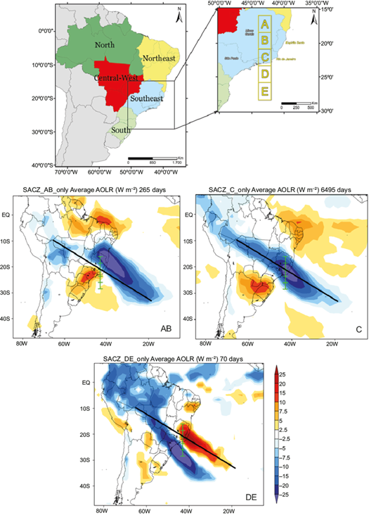
Fig. 1 The southeast of Brazil and the highlight for the AB, C, and DE regions of study (above). Longwave radiation anomalies for SACZ days at positions AB, C, and DE. The diagonal line represents the average position for reference (below). Source: Nielsen et al. (2019).
From this, to calculate the SACZ index, it is necessary to use the attributed weights for each variable to calculate the principal components and to perform a linear combination of the principal components to do the regression. All coefficients used in the steps of the SACZ index compose the methodology described and detailed by Nielsen et al. (2019). Thus, in each step, there are coefficients used to produce intermediate data, which will then be loaded into the calculation of the index. In summary, the SACZ index is calculated through the following steps:
Step 1: normalization of the input data.
Step 2: application of the weight of the principal components for each variable.
Step 3: linear combination of the principal components.
Step 4: logistic classification considering the thresholds h1, h2 and h3.
Results: output in csv with values of the SACZ index between 0 and 1 for the desired time period and a graphic plot to facilitate visualization.
Classification thresholds are important for the operational use of the index so that it facilitates the predictors’ decision-making by allowing a binary response (SACZ occurs/ SACZ does not occur) when the values are greater than/less than a given threshold.
To define the best cut-off thresholds, a range of values between 0 and 1 was used as thresholds and tested for sensitivity, specificity, and other metrics detailed in Nielsen et al. (2019) to define three main critical points (h1, h2, and h3) that will also be considered in this paper for region C (Table I).
Table I Thresholds for classifying SACZ events from the index for region C.
| Region | h1 | h2 | h3 |
| C | 0.14 | 0.34 | 0.52 |
Source: Nielsen et al. (2019).
To better understand the SACZ index classification, it is necessary to explain how the thresholds are interpreted. Threshold h1 represents the point at which the difference between the proportions of correctly and incorrectly classified events are maximal (it is the most sensitive threshold). However, the number of days with and without SACZ differ considerably between each other, so assessing the maximum difference in their proportions does not necessarily mean a positive difference with respect to the counting of days. Threshold h1, then, contemplates all historical SACZ events, however, it is the one with the highest number of false alarms.
The threshold in which the number of correctly and incorrectly classified events is the same is defined as h2 (it is the intermediate threshold). Threshold h2 indicates the value of the SACZ index when the number of SACZ events is equal to the number SACZ’ false alarms.
Finally, the threshold defined as h3 is the most specific. It uses the difference between correct and incorrect positive classifications in terms of absolute days rather than proportions. Thus, the SACZ index classification threshold h3 may not cover all SACZ events as the threshold h1 would, but it indicates the occurrence of the SACZ since the number of false alarms is minimal.
Values in Table I for the study region C allow an objective response from the SACZ index in terms of classifying a SACZ event. The lower threshold h1 = 0.14, the intermediate threshold h2 = 0.34, and the upper threshold h3 = 0.52 are identified as critical points and can be used as key values for the operational predictive use of the SACZ index to avoid the use of an arbitrary classification.
Thresholds h1 and h2 can represent perturbations of the atmosphere similar to the ones typical of SACZ events, indicating the presence of systems that can cause rainfall. Thus, they have great importance in the precipitation forecast in an operational environment, as the SACZ index makes the forecast independent of model parameterizations by evaluating only dynamic variables of the phenomena. Meanwhile, the h3 threshold (more specific) can represent the SACZ with its more defined dynamic configuration.
2.2 Comparison of SACZ events identified by CPTEC with the SACZ index in the 2017-2021 period
From the daily historical series of SACZ occurrence in reports and technical bulletins, events from 2017 to 2021 were selected to evaluate the capacity of the index to detect the phenomenon officially classified by CPTEC. Table II contains the start and end dates of the event according to the CPTEC report; the 15th date before the start of the event (I-15) to evaluate the forecast of the SACZ index with the input data from the GFS; the duration of the SACZ event and the predominant region of the SACZ (AB, C or DE) (Fig. 1).
Table II SACZ events notified by the Center for Weather Forecasting and Climate Studies (CPTEC) from 2017 to 2021.
| I-15 | Start | End | Duration | Region | I-15 | Start | End | Duration | Region |
| 2017-10-08 | 2017-10-22 | 2017-10-24 | 3 | C, DE | 2019-02-02 | 2019-02-16 | 2019-02-19 | 4 | AB, C |
| 2017-10-18 | 2017-11-01 | 2017-11-02 | 2 | AB | 2019-02-13 | 2019-02-27 | 2019-03-03 | 5 | C, DE |
| 2017-10-28 | 2017-11-11 | 2017-11-15 | 5 | AB, C | 2019-03-09 | 2019-03-23 | 2019-03-26 | 4 | AB |
| 2017-11-05 | 2017-11-19 | 2017-11-24 | 6 | AB, C, DE | 2019-03-26 | 2019-04-09 | 2019-04-11 | 3 | AB, C |
| 2017-11-14 | 2017-11-28 | 2017-11-29 | 2 | AB, C | 2019-11-02 | 2019-11-16 | 2019-11-19 | 4 | AB, C |
| 2017-11-17 | 2017-12-01 | 2017-12-15 | 15 | AB, C | 2019-11-22 | 2019-12-06 | 2019-12-08 | 3 | AB, C |
| 2017-12-16 | 2017-12-30 | 2017-12-31 | 2 | C | 2019-12-20 | 2020-01-03 | 2020-01-06 | 4 | AB, C |
| 2017-12-21 | 2018-01-04 | 2018-01-11 | 8 | AB, C, DE | 2020-01-10 | 2020-01-24 | 2020-01-28 | 5 | AB, C |
| 2018-01-16 | 2018-01-30 | 2018-02-09 | 11 | AB, C, DE | 2020-01-29 | 2020-02-12 | 2020-02-14 | 3 | AB, C |
| 2018-02-08 | 2018-02-22 | 2018-02-27 | 6 | AB, C | 2020-02-13 | 2020-02-27 | 2020-03-09 | 12 | AB, C |
| 2018-02-22 | 2018-03-08 | 2018-03-14 | 7 | AB | 2020-10-18 | 2020-11-01 | 2020-11-02 | 2 | AB |
| 2018-03-21 | 2018-04-04 | 2018-04-07 | 4 | AB, C | 2020-11-06 | 2020-11-20 | 2020-11-22 | 3 | AB |
| 2018-10-14 | 2018-10-28 | 2018-10-30 | 3 | AB | 2020-11-24 | 2020-12-08 | 2020-12-12 | 5 | AB, C |
| 2018-10-25 | 2018-11-08 | 2018-11-11 | 4 | AB, C, DE | 2020-12-09 | 2020-12-23 | 2020-12-25 | 3 | AB, C |
| 2018-11-05 | 2018-11-19 | 2018-11-21 | 3 | AB, C, DE | 2021-01-23 | 2021-02-06 | 2021-02-09 | 4 | AB, C |
| 2018-11-18 | 2018-12-02 | 2018-12-09 | 8 | AB, C | 2021-02-04 | 2021-02-18 | 2021-02-22 | 5 | AB, C |
| 2018-12-13 | 2018-12-27 | 2018-12-29 | 3 | AB, C | 2021-02-21 | 2021-03-07 | 2021-03-12 | 6 | AB, C |
| 2019-01-24 | 2019-02-07 | 2019-02-08 | 2 | AB, C |
The period of investigation comprises the months from October to April, the SAMS wet period, when SACZ is usually configured in the atmosphere (Carvalho et al., 2004). In five wet periods between 2017 and 2021, CPTEC recorded 36 SACZ events, including those with only 2 days duration.
2.3 Evaluation of the SACZ index as a prognostic tool
The main objective of this study is to answer how the SACZ index forecast performs with the GFS forecasts; that is, to evaluate the SACZ index as a statistically-based prognostic tool.
The forecast data chosen to be the input of the SACZ index was the GFS Global Model with a spatial resolution of 0.25º (NCEP, 2015), which is usually used as input for several regional models such as the Weather Research and Forecasting (WRF). The data was downloaded from the Research Data Archive (RDA) NCEP GFS 0.25 Degree Global Forecast Grids Historical Archive, for the months of October to April from 2017 to 2021 with the 00Z run, a discretization of 24 h, and a forecast horizon of 16 days (f000-f384).
For this study, the SACZ index calculation was done only for region C, which corresponds to the average position of the SACZ and covers the states of Rio de Janeiro and Minas Gerais in the southeast region, which suffer severe consequences as a result of the intense or persistent precipitation typical of the SACZ (da Fonseca Aguiar and Cataldi, 2021).
A widely used approach to quantify the degree of accuracy or agreement between estimated and observed values is the calculation of performance indices. According to the CPTEC definition for categorical evaluations, a tool elaborated by Wilks (2006) allows the comparison of forecast/observation pairs to be done through the data summary provided by the contingency table (Table III), in which it is possible to calculate metrics such as Probability of detection (POD), False alarm ratio (FAR), Accuracy, etc.
Table III Contingency table for calculating the indices’ performance evaluation.
| Contingency table | Observed | ||
| yes | no | ||
| Predicted | yes | A | B |
| no | C | D | |
Thus, based on the categories presented in matrix form (contingency table), it was possible to calculate some evaluation indexes:
-
Accuracy: indicates overall model performance; that is, among all classifications, reveals how many were classified correctly by the model. It is calculated using Eq (1):
-
POD: proportion of times that the event occurred and was correctly predicted; the higher the POD value, the better the model’s accuracy in predicting the event.
-
FAR: proportion of event predictions that turned out to be false alarms; the best possible value is zero (100% correlation with the observed) and the worst possible value is one:
From these evaluation metrics, we can compare the results between the observed SACZ index with Reanalysis II data, and the predicted SACZ index, calculated with GFS forecasts data. In this way it is possible to evaluate how many days in advance the SACZ index forecast can be used as a prognostic tool for forecasting the phenomenon in an operational environment.
In the next section, the forecast of the SACZ index with input from the GFS forecast data will be compared with the observed values of the SACZ index regarding the three defined thresholds (h1, h2, and h3). The results will be presented for each threshold. Then, the relation of the SACZ index considering only threshold h3 (more specific) it will be presented as a reference of the observed SACZ index data values, since it represents the occurrence of the SACZ with fewer false alarms.
3. Results and discussions
3.1 Comparison of CPTEC events with the index
Graphs were generated with the SACZ index values using input data from Reanalysis II from 2017 to 2021. Thus, it was possible to compare the records of SACZ events made by CPTEC (Table II) with the response of the SACZ index.
Figure 2 contains the plots of the index from 2017 to 2021 (until August) for region C. Analyzing the graphs in this figure, it is possible to observe higher values of the SACZ index at the beginning and end of the years, between the months of October to April, the wet period of the SAMS. Every event classified as SACZ by CPTEC was detected by the SACZ index. However, several of the peaks marked by the SACZ index did not enter the CPTEC technical bulletin, although the SACZ index response represents the presence of atmospheric dynamics typical of SACZ.
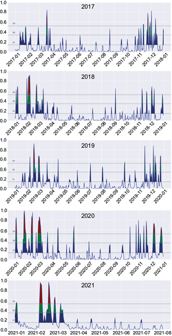
Fig. 2 Results of the SACZ index (Reanalysis II) in region C from 2017 to 2021 (until August). The blue shaded area indicates when the SACZ index values reached the h1 threshold; the green shaded area shows when the SACZ index values are higher than the h2 threshold, while the red shaded area indicates a SACZ index value higher than the most specific threshold h3.
Operational centers usually follow criteria for the detection of the SACZ, such as elaboration of a synoptic diagnosis and the combination of GFS variables to generate charts in GrADs and Gempak with cut-off thresholds defined according to the experience in the operational environment (Escobar, 2019). So, by using the SACZ index as a forecasting tool, it is possible to assist forecasters in operation and decision-making.
3.2 Performance evaluation of the index: results based on the NCEP GFS 0.25 forecasts (2017-2021)
Results of the SACZ index forecast from October to April for the period 2017-2021 were organized. Figures 3-7 show the values of each statistical metric for a given day of the GFS forecast above the thresholds h1, h2, and h3 over region C of the SACZ, from the analysis value (f000) to the forecast of 24, 48, 72, until 384 h (16th day of forecast). The results were arranged in graphs with the performance evaluation for the predicted (NCEP GFS 0.25 data) and observed (NCEP Reanalysis II data) SACZ index values (Figs. 3-7).
The h1 threshold is the lower classification threshold and considered the most sensitive (Nielsen et al. 2019). When analyzing Figure 3, it can be seen that up to the 9th forecast day, the POD of the SACZ index is always greater than 80%. Until the 10th forecast day, the FAR is less than 50%, with POD above 75% and Accuracy greater than 60%.

Fig. 3 Performance evaluation with POD, FAR, and Accuracy values of the SACZ index calculated above the most sensitive threshold h1, at region C, for October to April (2017-2021).
Although the probability of detection is always above 60% even on the 16th day of the forecast, FAR and Accuracy vary between 50 and 60% from the 11th to the 16th day. Considering the forecast of the SACZ index between October to April (2017-2021) and its lower threshold (h1), it is possible to determine that a good prediction of a SACZ event can be made until the 10th day of forecasting.
When the h3 threshold is considered as the reference for the observed index, the results shown in Figure 4 are obtained when there is the lowest number of false alarms of SACZ events (Nielsen et al., 2019) to compare with the SACZ index forecast from the most sensitive threshold (h1). By observing Figure 4, it is possible to notice that in the period 2017-2021 the POD of the SACZ index is always greater than 90% until the 8th day of the forecast. The probability of detecting a well-configured SACZ is approximately 68% in a 16-day (384 h) forecast. In the 16-day GFS forecast, Accuracy remains at about 64% (on day 1) and 48% (on day 16). The FAR increases accordingly with the increasing forecast horizon, ranging from 76% (on day 1) to 86% (on day 16).

Fig. 4 Performance evaluation with POD, FAR and Accuracy values of the SACZ index calculated above the most sensitive threshold h1, but considering as observed the h3 threshold, at region C, for October to April (2017-2021).
The intermediate threshold (h2) represents a stronger signal of a SACZ than the lower threshold (h1), but the number of correctly and incorrectly classified events is the same (Nielsen et al., 2019). Figure 5 presents the performance evaluation of the index from threshold h2.
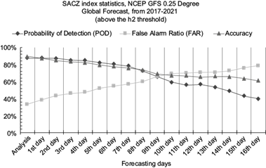
Fig. 5 Performance evaluation with POD, FAR, and Accuracy values of the SACZ index calculated above the intermediate threshold h2, at region C, for October to April (2017-2021).
When analyzing Figure 5, considering the intermediate threshold (h2), it is possible to observe that until the 4th day of the forecast, the FAR of the SACZ index is below 50%, and both the POD and the Accuracy are above 80%. Thus, a 96 h GFS forecast in the SACZ index can be considered a good forecast parameter that can ensure with a sufficient advance of days the detection of the dynamics of a SACZ or an event with similar dynamics. Both the POD and the Accuracy of the SACZ index in this case are always higher than 65% until the 9th forecast day.
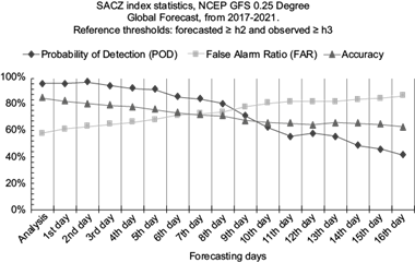
Fig. 6 Performance evaluation with POD, FAR, and Accuracy values of the SACZ index calculated above the intermediate threshold h2, but considering as observed the h3 threshold at region C, for October to April (2017-2021).
When considering threshold h3 as the reference of the observed SACZ index to compare with the SACZ index forecast from the intermediate threshold (h2), the results shown in Figure 6 are obtained.
Until the 5th day of the forecast, the POD of the SACZ index is always greater than 90%. The POD value is greater than 80% until the 8th day of the forecast. In the 16 days of the GFS forecast, the forecast accuracy remains approximately between 85% (on day 1) and 63% (on day 16). The FAR of the SACZ index increases along with the forecast horizon, ranging from around 58% (on day 1) to 87% (on day 16).
The most specific threshold (h3) represents a stronger signal of the SACZ configuration, i.e., it presents its most defined configuration, with the lowest occurrence of false alarms (Nielsen et al., 2019). The evaluation of the SACZ index for the study period is shown in Figure 7, according to which the FAR of the SACZ index surpasses 50% from the third day of the forecast. Until the 7th day of the SACZ index forecast, the POD remains above 70%, while Accuracy remains at a good value during all days of the forecasting, ranging from approximately 90% (on day 1) to 73% (on day 16).

Fig. 7 Performance evaluation with POD, FAR, and Accuracy values of the SACZ index calculated above the most specific threshold h3, at region C, for October to April (2017-2021).
If we consider the FAR as a “cut-off” metric, for the h3 threshold, a 72-h prediction in advance of a SACZ event indicates a good forecast of the SACZ index, with a RAF of approximately 50%, and both the POD and Accuracy greater than 87%. The FAR ranges from approximately 40% (on day 1) to 84% (on day 16) of the SACZ index forecast.
4. Conclusions
In this work, the SACZ index developed by Nielsen et. al (2019) has been adapted for use in weather forecasting from NOAA/GFS model results. In this way, the SACZ index has been validated to be used as a forecasting tool.
All comparisons were made by relating the predicted index with GFS data to the pseudo-observed index, calculated using the reanalyzes. The study by Nielsen et al. (2019) has already shown the correlation of the index with precipitation volumes during SACZ episodes.
When evaluating the metrics used in the contingency table for the average position of the SACZ (region C), the SACZ index between 2017 and 2021 revealed that from the lower and most sensitive threshold of the index (h1), the FAR is less than 50% until the 10th day of the forecast, with POD above 75% and Accuracy greater than 60%. When considering the threshold h3 as the reference for the observed SACZ index, when there are fewer false alarms of SACZ events, it was possible to observe that until the 8th day of the forecast, the POD of the SACZ index was always greater than 90%, and approximately 68% on the 16th day of the forecast (384 h).
When comparing the SACZ index forecast from the intermediate threshold (h2), considering the observed (h3) with the minimum false alarm cases of SACZ, it is observed that up to the 5th day of the forecast, the POD of the SACZ index is always greater than 90%, and this value remains greater than 80% until the 8th day of the forecast, with an accuracy ranging between approximately 85% (on the 1st day) and 63% (on the 16th day).
For the cases above the most specific threshold (h3), a 72-h ahead forecast of the SACZ index suggests an optimal forecast, with a FAR of less than 50% and both the POD and Accuracy above 87%.
For future works, we suggest the use of other atmospheric models as input for the SACZ index, such as the global model ECMWF or even the regional model WRF with higher resolutions. Additionally, we recommend an evaluation of the SACZ index from the perspective of different basic states, such as in El Niño, La Niña and neutral years.

