


 nueva página del texto (beta)
 Inglés (pdf)
 Artículo en XML
 Referencias del artículo
 Enviar artículo por email
 Citado por SciELO
  Similares en
SciELO
Similares en
SciELO 
 Permalink
1. Introduction
The advection-diffusion-reaction equation describes physical phenomena where particles, energy, or other physical quantities are transferred inside a physical system due to: advection, diffusion, reaction and forcing. This equation plays an important role in modelling the transport of a quasi-passive substance (for example, a pollutant) or a physical quantity (temperature, humidity, etc.) in the Earth’s atmosphere. In turn, the equations of nonlinear diffusion are widely used in modeling processes such as nonlinear combustion, rapid compression and accumulation of matter (laser fusion), chemical kinetics, magneto-hydrodynamics and many others. In particular, the fast-growing solutions of nonlinear diffusion equations can explain some important processes in demography (world population growth) and economics (rapid economic growth), meteorology (lightning and tornadoes) and ecology (growth of biological populations), epidemiology (outbreaks of infectious diseases) and neurophysiology, among others.
The quality of the general solution to the advection-diffusion-reaction problem strongly depends on the grids, discretization methods and the numerical algorithms used. In view of its great practical importance, the search for new directions for a radical improvement of the dissipative and dispersion properties of numerical schemes for this equation is an extremely urgent and fundamental problem in computational fluid dynamics. For example, in addition to the spherical (latitude-longitude) grids, there are other more complex variants such as the icosahedral (Majewski et al., 2002) or hexahedral (Giraldo and Rosmond, 2004) grids, which divide the spherical surface in a uniform way (or almost uniform way as in Majewski et al., 2002). These grids are not orthogonal, quite complex and have no relationship with spherical coordinates. On the other hand, they do not suffer from the problems associated with the presence of polar cells and are used with explicit schemes to reduce the restrictions on the time grid step to satisfy the Courant stability condition. For a more in-depth review of this topic, see Pudykiewicz (2006) and Staniforth and Thuburn (2012).
When discretizing in time, explicit or implicit numerical schemes are used. The explicit schemes are easier to implement, but conditionally stable. The stability condition imposes a restriction on the time step of the numerical scheme, which is not very convenient for long-term time integration. In turn, implicit numerical schemes, although unconditionally stable, require solving a system of linear equations at each time step. In the case of a multidimensional advection-diffusion-reaction equation, this approach requires the use of iterative methods, which significantly increases the computational time.
Our main goal was to develop an implicit and unconditionally stable numerical algorithm that is based on component-wise splitting of the problem operator and quickly implemented by direct (non-iterative) methods. The algorithm was developed and described in detail in Skiba (2015). This finite volume method differs significantly from the implicit finite-difference method previously proposed by Skiba and Filatov (2012, 2013, 2017). In what follows, we will call them the S-method and the SF-method, respectively. Both methods use the operator splitting, but the SF-method excludes from consideration both polar cells, thereby avoiding the challenge of imposing suitable boundary conditions. The highlight of the SF-method was the use of different coordinate maps of the sphere at the stages of splitting in the latitudinal and longitudinal directions. As a result, although the sphere is not a doubly periodic domain, all 1D split problems, both in latitude and longitude directions, are solved with periodic boundary conditions using Sherman-Morrison’s formula and Thomas’s method.
The S-method considers the pole cells and provides full and accurate coverage of the sphere by mesh cells (similar to icosahedral and hexahedral grids). This is especially important for solving advection-diffusion problems when an accurate description of flows near the poles and through the poles is required. The highlight of the S-method is the use of special bordered matrices for direct (non-iterative) solving the 1D problems arising at splitting in the latitudinal direction. The bordering procedure requires a prior determination of the solution at the poles.
The results of the first test calculations by the S-method, presented in Cruz-Rodríguez et al. (2019) and Skiba et al. (2020), showed the correctness of modeling processes near the poles and across the poles, an accurate description of the mass balance of matter in forced and dissipative discrete systems, and the conservation of the total mass and the solution norm in unforced and non-dissipative systems. The splitting method made it possible to create a direct (non-iterative) method for fast implementation of an implicit unconditionally stable algorithm, which is very important for long time integration of non-stationary problems.
Unlike the previous works, in this article, various linear and nonlinear problems are solved using the S-method on the high-resolution spherical 0.25º × 0.25º mesh.
2. Advection-diffusion-reaction model on a sphere
Consider the advection-diffusion-reaction problem on a two-dimensional sphere S:
where
Ag
= div (ug),
Dg
= -div (µ
and
where ſ S gdx is the total mass of the substance, and ǁgǁ = {ſ S g 2 dx}1/2 is the norm of the solution. Thus, both values increase if f > 0 and decrease under the influence of dissipative processes (σ > 0 or/and µ > 0). In particular, if f = µ = σ = 0 then
3. Brief description of the discrete model and numerical algorithm
The spatial discretization of Eq. (1) by the finite volume method was described in detail in Skiba (2015). The semi-discrete problem
approximates the differential problem (1) with the second order of accuracy in both
spatial variables. Here
Problem (1) is solved in the time interval (0, T) using the regular spherical grid with step τ and nodes t n = nτ (n = 0, 1..., 2N). In each doubled time interval (t n-1 , t n+1 ) , n = 1, 3, 5..., 2N - 1, Eq. (5) is solved by the symmetrized method of component-wise splitting of Marchuk (1982) using the Crank-Nicholson scheme for time discretization of 1D split equations:
Where
Denote f→[n] = f→(tn), g→[n + 1] = g→(tn+1) and g→[n - 1] = g→(tn-1) (n = 1, 3, 5...N - 1). Then the time discretization of each equation of system (6) using the Crank-Nicholson scheme leads to an implicit scheme
where the solutions
The scheme (7) of the S-method is implicit and unconditionally stable. In the case of
linear problems, it has a second order of approximation in time if
0.5τ ǁ
One of the important advantages of the implicit S-method is that it is implemented by
efficient direct methods without using iterative processes when solving systems of
linear equations at all stages of the splitting algorithm. In more detail, the 1D
split problems in the λ-direction are periodical and effectively solved using the
formula by Sherman and Morrison (1950) and
the factorization method by Thomas (1949).
And when solving the 1D split problems in the
4. Results and discussion
We now describe the results of solving both linear advection-diffusion problems and nonlinear diffusion problems on the high-resolution spherical 0.25º × 0.25º mesh using the S-method.
4.1. Linear problems
4.1.1. Pure advection problem: Role of the high-resolution mesh
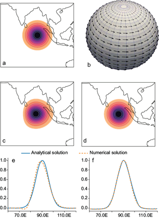
Let f = µ = σ = 0. Then we consider the pure advection problem
The initial condition g
0
(x) in the form of a spot and the zonal velocity
u
(x) = {u, 0} (super-rotation flow) are shown in
Figures 1a and 1b, respectively. In
this case, the solution must move in the zonal direction at the speed
u, while maintaining its original shape. At the moment
t = 5, the numerical solutions of this problem obtained
on two spherical grids with resolution 0.5º × 0.5º and 0.25º × 0.25º are
shown in Figures 1c and 1d,
respectively. Note that t = 5 is the dimensionless time it
takes for the initial spot to make a complete revolution around a sphere of
unit radius (Williamson et al.,
1992). The corresponding cross sections of these solutions
g(λ,
4.1.2. Linear advection-diffusion problem: Dispersion of a pollutant
The need to accurately predict the pollution levels and make operational decisions to overcome the consequences of pollution aroused a great scientific and practical interest in mathematical modeling of the processes of environmental pollution by anthropogenic sources.
We now apply the S-method to solve the linear problem of advection and diffusion of a passive substance (such as a pollutant) in the Earth´s atmosphere (a = 6371 km) with a non-divergent wind velocity u(x) obtained from the ERA5 reanalysis data (Fig. 2).

Suppose that g0(x) = 0, and dispersion of the substance g(x, t) occurs with µ = const and from the sixteen point sources whose location is marked by dots in Figure 3 at t = 4 days. We take σ (x, t) ≡ 0, since the reaction process is simple and only exponentially reduces the solution amplitude and norm with time. Similar assumptions were considered in the sections “Elliptic problem” in Skiba (2015) and “Spiral waves” in Skiba et al. (2020).
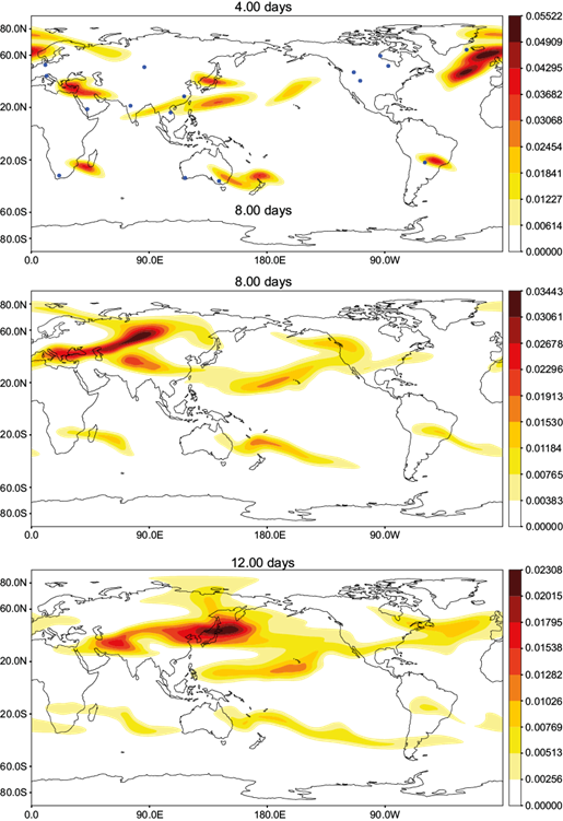
The sources emit the substance only during the first day:
and Qi = const is the intensity of emission of the i-th source. During the first day, the plumes of substance g(x, t) spread downwind, increasing their areas under the influence of diffusion. However, due to the effect of non-zero forcing, the plumes remain “attached” to the sources. From the second day onwards, the sources cease to emit, and the plumes leave the sources, propagating only under the influence of wind and diffusion. Figure 3 shows the positions of the substance plumes at t = 4, 8 and 12 days. Note that the S-method correctly describes the advection and diffusion of passive matter on the sphere. The same method makes it possible to effectively solve three-dimensional (3D) problems by adding splitting steps in the vertical direction to the splitting schemes (6) and (7), without changing the spherical part of the schemes. Furthermore, one can use the sigma-coordinate system and include the topography of the bottom. As a result, the 3D S-model will be useful for problems in oceanography, meteorology and other areas where hydrodynamics is important.
4.2. Nonlinear diffusion problems
The nonlinear forms of both diffusion coefficient and forcing are typical for plasma physics, chemical kinetics, destruction of plasticity, ecology, biology, medicine, etc. (Bekman, 1990; Glicksman, 2000; Skiba and Filatov, 2017; Vorob’yov, 2003). There are still many unresolved problems in those areas. In particular, the following questions are of interest: How and under what conditions do organized structures (vortices, solitons, dissipative structures) that are capable of self-sustaining for a finite time, appear in a homogeneous medium? How do they work and how do they evolve over time? Why do only certain types of structures arise, how is the spectrum of these structures arranged? How does the “complexity of the organization of a nonlinear dissipative medium” occur?
Let us now consider the nonlinear diffusion problem
This is a particular case of problem (1) if u (x,t) = 0, σ = 0, and
The second term in Eq. (8) describes the mechanism of non-linear diffusion; in addition, the diffusion coefficient depends on the solution according to a non-linear law. The term on the right side of Eq. (8) describes the energy release process. In fact, this is the power of the source. The intensity of the source depends on the solution according to a non-linear law.
Nonlinear diffusion is a scattering factor that attempts to smooth out inhomogeneities in the solution field. This term can be viewed as a sink of energy in the system, responsible for the creation of stationary structures. Nonlinear forcing tries to make the solution non-uniform and is the source of energy in the system. Energy sources are responsible for the creation of non-stationary (developing) structures. With nonlinear terms µ (g) and f (g), the system exhibits very complex behavior due to the incessant competition of two opposing processes. It is a self-organizing system that has an internal mechanism for the formation of structures and evolution (through nonlinear interactions and the realization of instabilities and bifurcations). Note that despite the complex behavior, the existing mechanism of asymptotic exit to relatively simple attractor structures, creates the possibility of prediction.
It should be noted that in the case of nonlinear terms (9), the only change that needs to be made to the numerical algorithm is the linearization of problem (8) at each doubled time interval (t n-1 , t n+1 ) setting
We also note that linearization reduces the order of approximation of the problem in time to O(τ).
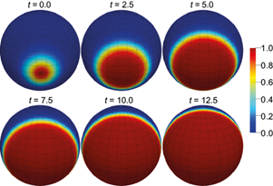
4.2.1. Self-sustaining temperature wave of nonlinear combustion
Despite the existence of examples of purely diffusion flame, in most of the observed combustion reactions, the main contribution to flame propagation is made by the heat source. For example, if
µ = const and f = α g - β g 3
Eq. (8) describes a family of nonlinear combustion processes , where solution g is the temperature. In this case, the term µ = const describes the mechanism of linear heat conduction, while the term f = α g - β g 3 is the power of the heat source. The intensity of combustion depends on the temperature according to a nonlinear law.
In particular, a self-similar solution arises, i.e., one in which the front of a non-linear wave of an unchanged shape moves at a constant speed. The case α = β = 1 is shown in Figure 4. We take
where ρ(x, x
0
) is the shortest distance between two points x and
x
0
on the sphere measured along the great circle connecting these points
(Skiba, 2017), a
= 1 and x
0
= (λ0,
4.2.2. Blow-up regimes of nonlinear combustion with positive strongly nonlinear feedback
In the previous experiment, we showed that the processes of accumulation and dissipation can generate a self-sustaining temperature wave of nonlinear combustion (Fig. 4). However, even more unexpected solutions of Eq. (8) are possible if the diffusion coefficient is also nonlinear.
Scientists are attempting to answer one of the important scientific questions, namely, “are there objective laws of evolution that are valid for complex systems of a very different nature: physical, chemical, biological and even for the human community and the person himself, his body, brain and consciousness?” Scientists’ intuition suggests that the blow-up modes describe the processes of evolution in complex systems of the most varied nature and have great commonality. They arise in nonlinear open dissipative systems with positive feedbacks. Such systems are autocatalytic reactions in chemistry, explosive modes in physics, free market mechanisms in the economy, information processes in society, mechanisms for the formation of social networks on the Internet, including in the global system of human society. All these evolutionary processes can be described by one model, which is based on a nonlinear heat conduction equation with a source. The nonlinear coefficient of thermal conductivity (diffusion) describes dissipative processes in the system, the propagation of the energy of matter or information, and the volume source describes cumulative processes, the rate of growth of energy, matter or information in the system. Accumulation and dissipation are the two most important dynamic components of processes in complex systems, and their incessant competition are the driving forces of evolution. The nonlinear dynamics of complex systems of different types can be considered in a unified way, from the point of view of the development and interaction of structures of different complexity, developing in a blow-up regime.
As an example, consider the case when
that is, problem (8) reduces to
If the production of a substance in each local area of the environment grows nonlinearly with its concentration in this area (as in our case where f = γ g β ), then the increasing concentration, accelerates the production of the substance. The presence of such positive strongly nonlinear feedback leads to instability when the deviations of the system from equilibrium increase over time. Due to the nonlinearity and the presence of a nonlinear positive feedback, an extremely rapid development of the process is possible (for various combinations of the parameters α > 0 and β > 0), when fast-growing solutions appear in a finite time (so called blow-up regimes or burning modes “with aggravation”).
To date, there are three well-known blow-up regimes that arise in one-dimensional nonlinear combustion problems with a power-law dependence of the forcing and the diffusion coefficient on the solution (Kurdyumov, 2006), in which a rapid increase in temperature can occur in an expanding combustion area (HS mode), in a reducing combustion area (LS mode) or in an unchanging combustion area (S mode).
In the case of the two-dimensional problem (10), we also simulated these
three blow-up combustion regimes on a sphere for different values of α and β
(see Figure 6): the HS mode, when the
temperature rises rapidly in the expanding combustion zone (Fig. 6a); the LS mode, when the
temperature rises rapidly in the narrowing combustion zone (Fig. 6b); and the S mode, when the
combustion process is always localized in the same area, while the
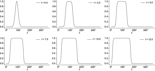
temperature is rising rapidly in a finite time (Fig. 6c). Figure 7
shows the cross sections g (λ,
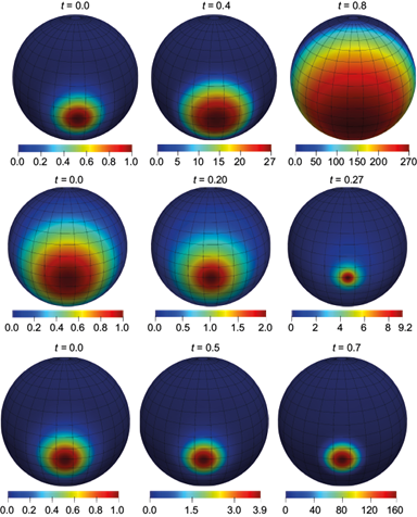
Fig 6 Blow-up regimes of nonlinear combustion for κ = 10-2, γ = 10,
g0 (x) ≡ exp {-C × ρ2 (x, x0)} and x0 = (λ0,
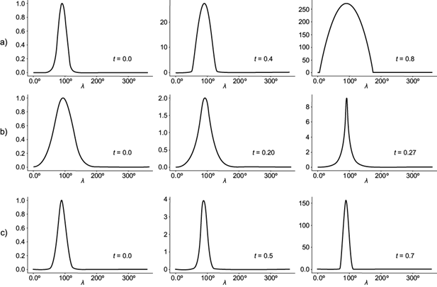
Fig 7 Cross sections g (λ,
In the HS mode, the combustion process initiated in the finite region propagates throughout the space. At the same time, it should be noted that one of the main results of the competition between nonlinear processes of heat transfer and heat release is the effect of localization of the combustion processes in the LS and S modes, which in these particular cases act as a manifestation of the self-organization process in a nonlinear dissipative medium.
It is clear that blow-up regimes are an idealization of real processes and do not consider the factors that limit the growth of the function under study near the blow-up moment. However, models in which solutions can grow in blow-up mode make it possible to understand and study the essential, most significant features of the system under study, which manifest themselves for a long time, up to until the aggravation moment. A remarkable feature of the theory of blow-up regimes is the presence of paradoxical properties in the simplest “classical equations” of mathematical physics.
If a problem admits an unbounded solution, then it is called globally (in time) unsolvable. The study of the spatiotemporal structure of unbounded solutions near the blow-up moment is associated with the wide use in the practice of physical experiments of various effects generated by ultrafast processes, for example, the effect of self-focusing of light beams in nonlinear media, the collapse of Langmuir waves in plasma, etc. The theory of blow-up regimes was extended to compressible media and the problems of dissipative and magnetic hydrodynamics. These results found an important application and experimental confirmation in the problems connected with laser thermonuclear fusion, in experiments on thermochemistry.
4.2.3. Self-organization processes in the Gray-Scott model
The production of materials of higher quality and maximum purity, and as a result the improvement of outdated technology, is vital due to competition from manufacturers. However, using only technological means, it is impossible to solve the emerging problems associated with improving product quality. There is a constant need for more and more perfect mastery of the various physical and chemical processes that play a decisive role at various stages of production. It is known that a significant part of the efforts now expended on chemical research is aimed at the synthesis of new compounds and the search for new reactions. Meanwhile, the study of the chemical process itself, the redistribution of bonds between reacting molecules, is gaining more and more scope. This is due to the fact that the possibilities of controlling a chemical process arise only when all parameters that determine the chemical process are found and analyzed.
Over the past several decades, chemical kinetics has given rise to many phenomena and mathematical problems. A classic example is the waves of the Belousov-Zhabotinskii reaction. One aspect of these systems is that they do not involve thermal transfer as an essential part of the interaction. One of such reaction-diffusion models is the nonlinear Gray-Scott model of a pair of reactions with cubic autocatalysis (Gray and Scott, 1994):
Here κ represents the rate of conversion of v to another chemical species, while ω represents the rate of the process that feeds u and drains u and v. Nonlinear positive feedback is an essential element in autocatalytic process models. Autocatalysis is the acceleration of a chemical reaction by one of its products.
It is known that the spatial Gray-Scott model with low diffusion coefficients of reagents shows not only a rich variety of self-replicating patterns of concentration profiles: bands, spots, waves (Pearson, 1993; Har-Shemesh et al., 2016), but also impressive examples of spatio-temporal chaos. In the case of spots, self-replication is visually similar to cell division in that an initially radially symmetric spot elongates into a peanut shape and then splits into two spots. However, the further evolution of the two daughter spots may be to any number of other patterns.
This paper presents four numerical solutions of the Gray-Scott model (11) on the sphere, obtained using the S-method. Note that the trivial state u(x, 0) ≡ 1 and v(x, 0) ≡ 0 always exists and is stable for all ω and κ. Therefore, we take the initial values u(x, 0) and v(x, 0) different from this state. They are shown in Figure 8a: u(x, 0) = 0.5 + q(x) and v(x, 0) = 0.25 + q(x) inside the square, while u(x, 0) = 1 + q(x) and v(x, 0) = q(x) outside the square. The function q(x) takes random values in the range [0, 5 × 10⁻²]; a = 114.59; κ = 0.25; µ = 0.16; χ = 0.08.
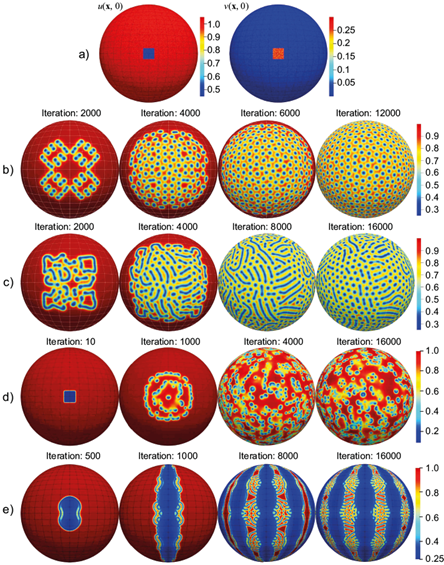
Fig. 8 Four numerical experiments with the Gray-Scott model. a) Initial conditions u (x, 0) and v(x, 0). b) u(x, t) for ω = 0.026, κ = 0.061; c) u(x, t) for ω = 0.030, κ = 0.060. d) u(x, t) for ω = 0.010, κ = 0.047. e) u(x, t) for ω = 0.030 + 0.035 sin (6ϑ)2, κ = 0.050 + 0.015 sin (6λ)2.
Numerical solutions of the Gray-Scott model produced some interesting patterns. Figures 8b-e show the field u(x, t) calculated for four different values of the parameters ω and κ. Note that κ is constant everywhere except for the last experiment (Fig. 8e), where κ is a function. In all experiments, nonlinear interaction, dissipation, and instability give rise to bifurcations (Nishiura and Ueyama, 2001) and, as a consequence, self-organization processes which manifest themselves in the appearance of various irregular spatio-temporal patterns. Their shapes depend on the initial conditions and internal parameters of the model such as µ, χ, ω, κ. For example, in Figures 8b and 8c, the newly formed structures very quickly move away from each other at a sufficiently large distance so that they become independent and then split themselves. As a result, the entire space is filled with motionless localized structures located at some distance from each other. The solution shown in Figure 8d resembles the appearance of chemical turbulence. Finally, the role of the spatial distribution of the diffusion coefficient on the spatial structure of the solution is shown in Figure 8e.
Figures 8b, 8c and 8d, along with the results of numerical experiments by Skiba et al. (2020) using a low-resolution S-model, show the structural instability of the Gray-Scott model with respect to small perturbations in the model parameters ω and κ. Indeed, depending on small variations of the model parameters ω and κ, the solutions approximate different attractors over time.
5. Conclusions
An implicit and unconditionally stable numerical method of the second approximation in space and time developed in Skiba (2015) is used here to solve linear advection-diffusion-reaction problems and nonlinear diffusion problems on a sphere. The first tests carried out in Cruz-Rodríguez et al. (2019) and Skiba et al. (2020) demonstrated that the method correctly models the processes of advection and diffusion near and across the poles and accurately describes the evolution of the total mass of matter in forced and dissipative discrete systems. They also confirmed that in the absence of external forcing and dissipation, the method preserves the total mass of the substance and norm of the solution. These characteristics are very important in long-term calculations, as for example, in the case of numerical experiments with the Gray-Scott model. Although the two-dimensional scheme is implicit, the method of splitting the problem operator allows us to construct a direct (non-iterative) numerical algorithm that is fast to implement. Numerical experiments, carried out in this work with a high-resolution model, show the precision and efficiency of the method, which makes it possible to accurately simulate global and local linear advection-diffusion processes on the sphere (such as dispersion of a pollutant, or transport of temperature or humidity), as well as nonlinear diffusion processes such as blow-up regimes of combustion, propagation of nonlinear temperature waves of combustion, and complex chemical processes described by the Gray-Scott reaction-diffusion model.
Note that the results shown in Figure 8, along with the results of numerical experiments by Skiba et al. (2020) using a low-resolution S-model, show the structural instability of the Gray-Scott model with respect to small perturbations in the model parameters ω and κ.

