


 nueva página del texto (beta)
 Inglés (pdf)
 Artículo en XML
 Referencias del artículo
 Enviar artículo por email
 Citado por SciELO
  Similares en
SciELO
Similares en
SciELO 
 Permalink
1. Introduction
Climate regionalization of the territory is essential for characterizing spatial and temporal climatic variability (Pineda-Martínez et al., 2007), producing meteorological forecasts, and analyzing trends at different scales based on the spatial homogeneity of phenomena. Regionalization also helps to ensure differentiated planning in the management of the territory’s water resources (Srinivas, 2013) and to measure the impact of climate change in different regions (Almazroui et al., 2015), thus contributing to better decision-making in the ordering and management of the territory (Virmani, 1980). The division of a territory into climatic subregions facilitates the study of the climatic impact on human activities, mainly due to the representation of extreme events such as floods and droughts (Seiler et al., 2014). These climatic subregions can also be used to link climatic information with the different physical and socioeconomic aspects needed for climate assessments, found at different spatial resolutions and levels of aggregation (Perdinan and Winkler, 2015). Other applications are also related to the study of crop yields associated with climatic variation in subregions (Araya et al., 2010; Borges et al., 2018; García-Barreda et al., 2019), as well as the global distribution and productivity of domestic livestock (White et al., 2001).
The regionalization of climatic phenomena is a challenging task when their spatial and/or temporal variability is high (North et al., 1982; White et al., 1991; Catell, 1996; Comrie and Glenn, 1998; Díaz and Mormeneo, 2003). Classification outcomes differ according to the variables selected, the methods used, and the data sets and time periods employed (Dambul and Jones, 2008). Therefore, delineation is usually performed according to specific objectives and on specific data sets such as extreme high or low rainfall on a monthly, daily, or hourly basis, and droughts, among others. Thus, concepts like the ‘regional homogeneity’ of areas resulting from a given delineation will not be the same for different objectives (Srinivas, 2013).
A substantial body of research has used different data sets to define climatic types and then delineate similar climatic zones. The most widespread examples worldwide are the Köppen (1923) and Thornthwaite (1931) classifications (Fovell and Fovell, 1993), which have been updated in recent years by other authors using more extensive climate series and higher density of meteorological stations (Feddema, 2005; Peel et al., 2007; Beck et al., 2018). Other studies have classified climate regimes by hydrographical basins, geographical boundaries, extent of major mechanisms of atmospheric circulation, and altitudinal divisions, among others (Korecha and Sorteberg, 2013).
For the province of Santa Cruz, in southernmost continental Patagonia (Argentina) where this work is focused on, the only known precedent for a climatic regionalization proposal, apart from the best-known world classifications (Köppen and Thornthwaite), is that of de Fina et al., (1968), which is based on thermal and pluviometric characteristics drawn upon multiple data sources. Using a total of 450 points in the province with records of more than 30 years, between the period 1921-1950, they defined a total of 41 agroclimatic districts. The large number of climates that this Argentine province offers is the result of the enormous extension it occupies, its notable differences in altitude, latitude, and complicated relief, making it the third province with the greatest diversity of agroclimatic regions, behind the provinces of Chubut and Mendoza (Defina et al., 1968).
Santa Cruz province exhibits strong climatic gradients, in which rainfall decreases from west to east and from south to north (Almonacid et al., 2021), while temperature decreases from northeast to southwest (Almonacid et al., 2022). In addition, the region has different areas characterized by their variation in landscape, with hills in the center of the province, river valleys, and coastal areas, as well as a western strip with a mountainous environment, each of which is associated with different plant species that respond accordingly to climate variability (Oliva et al., 2001; Peri et al., 2013). The province has large natural freshwater reserves, such as Los Glaciares National Park, located in the southwest, where part of the southern ice field is located, as well as other sources of freshwater originating in the Andes mountains, where the most important rivers that cross the province from west to east flow into the shores of the Mar Argentino. Such diversity in the region makes it necessary to create subregions based on the climate, which acts as a moderator of the interactions between water, soil, and plant species.
The main objective of this study is to propose a climatic regionalization for Santa Cruz province, based on gridded rainfall and temperature data, and their subsequent characterization. This climatic division for the province will be of great importance for future analysis of extreme events in the region such as extreme rainfall events, extreme temperature, extreme winds, snow, and droughts, as well as evaluation of climate risks, in addition to the study of climate change and its effects on natural systems in subregions with similar climatic characteristics.
2.1 Study area
Santa Cruz province is located to the south of continental Patagonia, Argentina, between the parallels 45º-53º S and 65º-72º W (Fig. 1). The latitude, altitude, and proximity to the Mar Argentino of the different areas of the province determine patterns in the climate, in particular the spatial variability of rainfall and temperature (Almonacid et al., 2021, 2022).

Fig. 1 Topography of Santa Cruz province and its administrative boundaries. White circles represent the main cities in the province.
Santa Cruz is characterized by a highly variable relief, with heights between 0 and 100 masl in the coastal area to the east (Fig. 1), a central area with heights above 500 masl, and the presence of the Andes mountain range towards the west of the region, with a north-south distribution and altitudes between 1200 and 3900 masl. The Andes mountains act as an orographic barrier blocking the disturbances embedded in the westerly flow and consequently the humid air masses from the Pacific Ocean (Insel et al., 2010; Bianchi et al., 2016), producing hyper humid conditions on the west side of the Andes and dry conditions on the eastern side (Garreaud et al., 2013). In the region of study, this barrier causes a considerable pluviometric gradient, with values over 1200 mm year-1 on the border between Argentina and Chile, with absolute extremes ranging from up to 9,000 mm year-1 on the continental ice fields (Sauter, 2019) to 200 mm year-1 towards the Atlantic coast (Almonacid et al., 2021). The north-central region of the province is the driest, with rainfall not exceeding 150 mm year-1. However, the Andes in this region, in general, do not exceed 3 km in height and subsequently, the Pacific air masses can dominate in the region (Labraga and Villalba, 2009). In addition, precipitation presents large variability in different time scales. The seasonality of rainfall depends on the geographical location, while the southeast of Santa Cruz presents higher rainfall in the summer, the western region near the mountain range shows the lowest seasonality, with values between 100 to 150 mm year-1 throughout the four seasons (Almonacid et al., 2021). One relevant phenomenon that influences precipitation variability on the intra-seasonal and intra-annual scales is the frontal activity in the region in connection with the variability of the atmospheric circulation patterns (Blázquez and Solman 2016, 2017). On decadal and interdecadal scales there is a relevant oceanic influence on the precipitation in the region of study, via Rossby wave trains (Berman et al., 2012).
The spatial pattern of temperature is mainly determined by the north-south latitudinal gradient and elevation (Villalba et al., 2003). The Andes mountain range also introduces changes in the spatial pattern of temperature through the release of adiabatic heat from the Pacific air masses as they descend from the mountains (Bianchi et al., 2016). The warmest zone in Santa Cruz is the northeast, with mean annual temperatures between 10 and 13 ºC, while the coldest climate occurs towards the west and south, with mean annual values between 6 and 8 ºC (Almonacid et al., 2022). The greatest spatial differences in mean monthly temperature are recorded for January (the warmest month), with a variation range of over 5 ºC, exhibiting a maximum of 16.7 º C in the northeast of the province and a minimum of 11.4 ºC towards the south, on the border with Chile (Almonacid et al., 2022). In July (the coldest month), these differences are smaller, with a variation range of 3.7 ºC, a maximum of 3.8 ºC and a minimum of 0.1 ºC for the same regions, respectively.
2.2 Database
The spatial and temporal variation in rainfall and temperature was analyzed using the gridded temperature and precipitation databases for Santa Cruz (GTDSC and GPDSC), created by Almonacid et al. (2021, 2022) for this province. These databases have the monthly mean values of both variables for the period 1995-2014, with a spatial resolution of 20 km. The GPDSC and GTDSC were created from the geostatistical spatial interpolation technique known as kriging. For the construction of both databases (GTDSC-GPDSC), records were obtained from official meteorological stations belonging to the National Meteorological Service of Argentina (NMS), National Institute of Agricultural Technology (NIAT), General Directorate of Waters (GDW) of Chile, as well as other unofficial stations belonging to private agricultural establishments and mining companies among the most important. In the case of the GPDSC, a total of 42 stations were used, while for the GTDSC, 36 stations were used.
These databases showed satisfactory results for the region, in comparison with other global databases (CRU, ERA5, UDEL, PERSIANN, and TERRACLIMATE), showing better performance in representing the spatiotemporal variation in rainfall and temperature in Santa Cruz province (Almonacid et al., 2021, 2022). To carry out the performance evaluation of these climatic databases, the authors used indices such as percentage mean deviation (PBIAS), relative mean absolute error (RMAE), and relative root mean square error (RRMSE), obtaining better indicators for rain and temperature than global climatic databases (Almonacid et al., 2021, 2022). GPDSC and GTDSC cover a geographic scope beyond the administrative boundaries of Santa Cruz province, reaching the south of Chubut, and regions sharing water resources with Chile, representing a total of 934-pixel centroids. In the present work, the total centroids were used for a better interpretation of the border situation.
Most of the databases validated in the region were created using data from meteorological stations; therefore, the best representation of the climatic variables is found in areas close to the meteorological stations that provided the primary data. For this reason, the main drawback of these global or quasi-global databases lies in the difficulty of properly representing the variability in rainfall and temperature in areas with low density of meteorological stations, which is even more difficult in areas with a high gradient such as the Andes mountains (Bianchi et al., 2016; Almonacid et al., 2021, 2022).
2.3 Zoning methodology
Twelve mean monthly averages (1995-2014) were obtained from each gridded database (rainfall and temperature), which maintained the original density and distribution of the respective grids, representing a total of 934 grid points (observations) within the scope of the gridded databases.
For the grouping of these observations, the statistical clustering technique was used, in which all observations are subdivided into smaller groups with some similarity to each other (Abadi et al., 2020). The most common techniques include hierarchical and non-hierarchical clustering. Both are widely used in atmospheric sciences, each having its advantages and disadvantages (Fovel and Fovel, 1993). In this study, non-hierarchical clustering was selected, as it is widely used in hydroclimatology studies, due to advantages like effective computations, simple mathematical basis, and easy implementation (Bhatia et al., 2020).
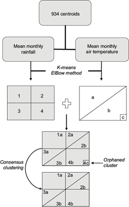
Non-hierarchical clustering, better known as k-means clustering, randomly assigns observations to a predetermined number of clusters. Then, the internal error of each cluster is computed by the within-cluster sum of squared (WSS) errors (Eq. [1]) that is computed as a sum of the squared distance between each observation of the cluster and the cluster centroid (Euclidean distance). These observations are then repeatedly reassigned to clusters with a closer centroid, followed by the recomputing of these centroids, until an optimal approximation is reached. In this approach, closer observations have more influence on each other. One of the main disadvantages of this method is the need to establish a priori the number of climatic clusters or regions (Carvalho et al., 2016). For a variety of analytical processes and downstream uses of downscaling, it is desirable to propose as few climatic regions as possible to ensure easy interpretation and analysis of results and trends (North et al., 1982; White et al., 1991; Catell, 1996; Comrie and Glenn, 1998; Díaz and Mormeneo, 2003). Given the lack of precedents of climate regionalization in Santa Cruz, an approximation to the possible number of clusters was tested using the within-cluster sum of squared error technique, which makes it possible to compute the sum of squared distances between each member of a possible cluster of clustered data and the corresponding centroid (Abadi et al., 2020). If k is defined as the number of target clusters for regionalization, starting at 1 and up to n, we proceed to calculate the error of the distances, which decreases as k increases. This tends to stabilize after reaching an optimal k (better known as the “elbow” or inflection point in the curve), which can be selected as a possible k to establish the clustering level. In this case, the elbow technique is used to select the final number of clusters for rainfall and temperature, where the inflection point on the curve determines the optimal value of k.
where k is the cluster number, n the number of cases, xi the i case and Cj the centroid for cluster j. For the calculation of these statistics, the student version of the InfoStat software was used.
On the other hand, selecting the appropriate climate variables is the precondition for achieving an accurate and useful climate classification (Chen et al., 2009; Darand and Daneshvar, 2014). Several authors point to rainfall and air temperature as the climate variables that best define the climate of a region (Fovell, 1997; Almazroui et al., 2015; Carvalho et al., 2016; Abadi et al., 2020). In general, their records are usually greatly generalized and easily available in wide regions of the world. Even where other records are usually absent, they have great spatial and temporal variability and are strongly correlated with other relevant climatological phenomena, making them good predictors. In addition, their dynamic is central to nature and society, mainly because they condition the natural supply of surface water and underground recharge (Chen et al., 2009; Darand and Daneshvar, 2014).
The rainfall variable was transformed to minimize potential errors given the great spatial variability. To achieve this, the square root transform technique was applied to mean monthly rainfall, since it naturally follows a gamma distribution (Richman and Lamb, 1985). This was not applied to temperature since it follows a normal distribution (Abadi et al., 2020).
Once non-hierarchical clustering was applied for grouping each climatic phenomenon, both were combined to obtain climate regions based on their thermal and pluviometric characteristics. Considering that a number of m groups for rainfall and n groups for temperature can be formed, then a maximum of m × n possible climatic categories can be formed, which requires a subsequent reanalysis to eliminate inconsistencies and excessively small clusters or clusters lacking representative data. For cluster simplification, Fovell and Fovell (1993) proposed an approach called consensus clustering by means of which subcategories based on the intersection of individual clusters can be created. The authors also showed that intersections near the boundaries of a region create small “orphaned” clusters made up of few observations, not large enough to be considered a distinct climatic region. When these clusters occurred, they were reassigned to larger neighboring clusters that allowed the final number of regions to be simplified and made it feasible and simple to interpret and characterize. Figure 2 show a summary of the methodologies used for climate regionalization.
2.4 Classification of climate regions
Once the climate clusters were obtained, the Thornthwaite classification modified by Feddema (2005) was used to classify each cluster. This method was used in order to assign a known climatic classification to the clusters obtained. This classification distinguishes climate types based on two primary factors, moisture, and heat, in addition to the use of two seasonality components as the second factor. For the classification of the present study, only the primary factors were used, because this region does not present such marked seasonal gradients, as it happens in other parts of the world, where, for example, monsoon-type rains occur in limited periods of the year.
The moisture factor is a concept created by Thornthwaite to replace the direct use of rainfall with the concept of potential evapotranspiration (PE). The PE (Eq. [2]) is based on temperature and day length to estimate the water need of plants in a given environment.
where T is the mean monthly air temperature expressed in ºC,
Using PE in combination with rainfall, Thornthwaite developed the water balance methodology to create a moisture index (Im) (Eq. [3]). According to its adaptation by Feddema (2005), this index can take values between 1 and -1, whereby values close to -1 indicate a lack of rainfall, while values close to 1 indicate a lack of evapotranspiration. The second classification concept is the thermal factor related to the productivity of an environment, where Thornthwaite uses PE as a predictor. To complement Thornwaite’s classification, the mean temperatures of the coldest month and the warmest month were used to assign a different climate type to each cluster obtained (Feddema, 2005).
3. Results
3.1 Clusters selection
The calculation of the within-cluster sum of squared errors, from k = 2 to k = 14, yielded a significant reduction in the first four clusters. The inflection point for each variable was obtained for k = 5, indicating the optimal number of clusters according to the elbow method (Fig. 3a, b). However, for rainfall, only three clusters were found within the provincial borders (Fig. 3d), the other two being associated with regions of abundant rainfall in Chilean Pacific areas. On the other hand, for temperature, each of the five clusters formed was represented in the study region (Fig. 3c). The results found with the elbow method are geographically consistent. Besides, an independent sensitivity analysis to cluster numbers was performed (not shown), which evidences that the selection of cluster numbers larger than k = 5 does not generate a differentiation of a greater number of areas of climatic interest.
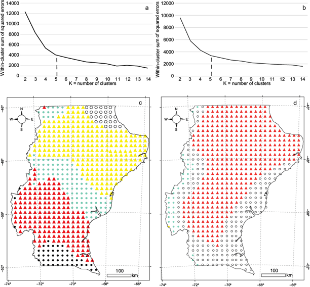
Fig. 3 Within-cluster sum of squared errors for (a) temperature and (b) rainfall. Regionalization based on the (c) mean monthly temperature and the (d) mean monthly accumulated rainfall for Santa Cruz province.
The clusters obtained from the mean monthly temperature (Fig. 3c) were able to replicate the behavior of the main isotherms analyzed by Almonacid et al. (2022), where predominant latitudinal distribution is evident in the separation of different zones. For rainfall, zoning follows the behavior of the annual isohyets, with a central zone with lower mean annual rainfall (MAR), between 130 to 200 mm year-1, an evident coastal zone, and a small strip to the west of the province, with a MAR between 200 and 300 m year-1. And, finally, a western zone, close to the Andes mountain range, with a MAR between 300 and 500 mm year-1.
3.2 Climate regions
After cutting across the different clusters formed for rainfall (n = 3) and temperature (m = 5), 13 of the 15 potential climate regions (n × m) were confirmed. Two regions had only one isolated pixel and were reassigned to a closer higher climate region to reach a final clustering of 11 climate regions classified following Thornthwaite’s method modified by Feddema (2005) (Fig. 4).
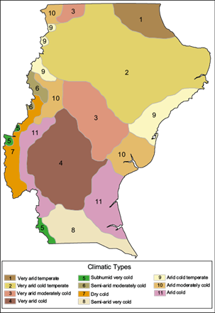
Fig. 4 Spatial distribution of the 11 climate regions and their classification according to the Thornthwaite method modified by Feddema (2005).
Zones 1, 2, 3, and 4 were found to be very arid zones (Table I), differentiated between them by the temperature gradient. Temperature decreases towards the south, where the warmest region is located to the northeast, with the highest thermal factor of 780 mm year-1 of PE and a mean annual temperature (MAT) of 11.7 ºC (Fig. 5). In contrast, the zone located further south (zone 4) is classified as cold, according to the thermal factor, with 510 mm year-1 of EP and a MAT of 7.4 ºC. These areas have a humid season from May to August (Fig. 5) and a predominantly dry season the rest of the year, more noticeable to the northeast of the province.
Table I Classification of the climate regions for Santa Cruz province according to Thornthwaite (adapted by Feddema 2005) and mean values of the temperature of the coldest and warmest months as a complement in the discrimination of regions.
| Zone | Thermal factor1 | Moisture factor2 | Climate classification according to Thornthwaite3 | Mean temperature of the coldest and warmest month |
| 1 | +700 | -0.83 to -0.66 | Very arid temperate | |
| 2 | 600 to 700 | -0.83 to -0.66 | Very arid cold temperate | |
| 3 | 500 to 600 | -0.83 to -0.66 | Very arid moderately cold | This region is characterized by presenting an average temperature in January > 14 ºC and an average temperature in July > 1.8 ºC. |
| 4 | 500 to 600 | -0.83 to -0.66 | Very arid cold | |
| 5 | 400 to 500 | 0 to -0.17 | Subhumid very cold | |
| 6 | 500 to 600 | -0.5 to -0.33 | Semi-arid cold | |
| 7 | 500 to 600 | -0.33 to -0.17 | Dry cold | |
| 8 | 400 to 500 | -0.5 to -0.33 | Semi-arid very cold | |
| 9 | 600 to 700 | -0.66 to -0.55 | Arid cold temperate | |
| 10 | 500 to 600 | -0.66 to -0.55 | Arid moderately cold | This region is characterized by presenting an average temperature in January > 14 ºC and an average temperature in July > 1.8 ºC. |
| 11 | 500 to 600 | -0.66 to -0.55 | Arid cold |
1Annual potential evapotranspiration in mm year-1; 2moisture index (Feddema, 2005); 3table adapted from Feddema (2005).
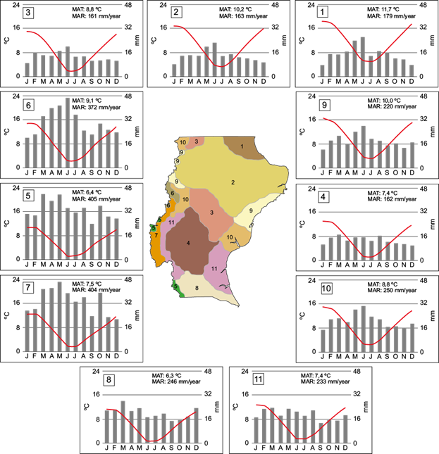
Fig. 5 Climographs of the 11 climate regions classified for Santa Cruz province with their mean annual rainfall (MAR) values (mm year-1) and mean annual temperature (MAT) values (ºC).
As it was expected, the most humid areas were located towards the west of the region (zones 5 and 7), where the midlatitude waves, embedded in the westerly flow (with a maximum between 45-55º S), cross the Andes (Garreaud, 2009). Zones 5 and 7 have the highest annual rainfall (405 and 404 mm year-1, respectively), the former being the coldest with a mean annual temperature of 6.4 ºC. These two climate regions exhibited a humid season throughout most of the year, more prominently so in zone 5 (subhumid cold). These regions are associated in the province with zones of ñire (Nothofagus antarctica) and lenga (N. pumilio) forests, the main native forest species in the province.
Zones 6 and 7 displayed higher rainfall in autumn and winter, unlike the other regions, where a seasonal component in rainfall was not so marked (Fig. 5). Furthermore, zone 6 presents an average annual rainfall of 372 mm year-1, being a little lower than zones 6 and 7, presenting instead a higher average annual temperature than the two mentioned zones (9.1 ºC). According to the climogram presented in Figure 5, this area presents a water deficit in the summer months.
The coastal area of the province was mainly represented by climate zones 1, 2, 8, 9, 10, and 11, with mean annual rainfall between 160 and 180 mm year-1 for the two northern coastal areas of the province (zones 1 and 2) and between 220 and 250 mm year-1 for the zones located towards the south coast of the province (zones 8, 9, 10, and 11), where the main difference between them was the mean annual temperature, decreasing towards the south (zone 8) and reaching 6.3 ºC. One singularity of these areas is they can be influenced by sea breezes, which develop due to the differential heating of air over coastal areas and the adjacent seawater. This mesoscale phenomenon strongly affects wind circulation and temperature patterns softening seasonal variability (Pessacg et al., 2021).
On the other hand, intense rainfall in coastal areas can be influenced by Atlantic moisture transport. In general, the few rainfall events in extra-Andean Patagonia are related to frontal systems and cyclone activity due to troughs from the Pacific, however, in coastal areas anomalous presence of easterly winds along the coast could influence the rainfall events (Agosta et al., 2019, 2020).
Besides, it is relevant to mention that zone 8 is one of the main ones in extensive sheep production, characterized by the presence of highly productive grasslands, while in the regions located further north (with less average annual rainfall and higher average annual temperature) the production of consumable grasses by sheep is lower. This increases the number of species adapted to drought conditions, such as creeping subshrubs and shrubs with deeper roots, which allow them to explore the water in lower layers (Oliva et al., 2001).
Zone 2 is the largest in the province. In addition to occupying a coastal area to the north, it extends over most of the northern-central zone, a hilly environment with a continental influence. This central area of the province was found to be the most arid, with mean annual rainfall not exceeding 160 mm year-1, where zone 2 also has the highest mean annual temperature (slightly over 10 ºC).
4. Discussion and conclusions
In the present study a climatic regionalization for Santa Cruz province, based on gridded data of rainfall and temperature, was performed. Application of the k-means method showed good results in clustering homogeneous climatic areas, both for temperature and rainfall, following in both cases the behavior of the main isotherms and isohyets of the region. The statistical regionalization method made it possible to delineate 11 homogeneous climate regions for Santa Cruz province, yielding the driest and warmest regions in the center and northeast and the most humid and coldest ones in the south and southwest. Most of the study region is classified as very arid, represented by regions located in the central part of the province with continental characteristics (climate regions 1, 2, 3, and 4) where the average annual rainfall regime is between 161-179 mm year-1. These regions differ from each other by their mean annual temperature, with the gradient decreasing as we move further south. The rainiest regions are those representing the smallest area in the province (located to the west, accordingly with the rain shadow effect eastward of the Andes); they are classified as subhumid (R-5) and dry (R-7), both with an average annual rainfall close to 400 mm year-1 and a temperature annual average between 6.4-7.5 ºC. On the southern border with Chile is the coldest region (R-8), classified as semiarid very cold, with a mean annual rainfall of 246 mm year-1 and a mean annual temperature of 6.3 ºC. The rest of the regions (9, 10, and 11) are distributed in space with a variant close to the Mar Argentino and oceanic influence, and another geographical component associated with the western part of the province close to the Andes mountain range. In these arid regions the average annual rainfall exceeds 220 mm year-1 with an annual average temperature between 10-8.8 ºC.
The k-means methodology proves to be efficient in separating the more humid areas in the south and west from those less humid in the center and north, as well as the warmer ones in the north from the colder ones in the south and west, evidencing the good performance of the algorithm of clusterization for the subdivision of the territory and showing results similar to Abadi et al (2020), who were able to divide Bolivia according to its climatic characteristics, separating the most important climatic regions. Other authors using the same methodology also achieved good results in the division of climatic regions based on temperature and precipitation (Fovell, 1997; Carvalho et al., 2016).
The only precedent of climate regionalization in the Santa Cruz province, performed by de Fina et al. (1968) using 450 points with records of over 30 years (spanning from 1921 to 1950), defined climate zones based on the mean temperature of the warmest month of the year (January), that of the coldest month (July), the mean rainfall of the hottest quarter (December, January, and February), the mean rainfall of the coldest quarter (June, July, and August) and the percentage of rainfall in the remaining semester relative to the previous one, yielding 41 agroclimatic districts. Despite the similarities with our study (more humid areas in the strip close to the Andes mountain range with mean annual rainfall values exceeding 500 mm), the present work updated the climate data series, expanded the number of input variables, and simplified the climate regions to a smaller number, thus facilitating decision-making on the territory. Although this update in climatic data, our work presents the limitation of using gridded databases that represent an average of only 20 years of data, with a minimum of 30 years recommended. Another limitation related to the databases used is the uncertainty they present in areas with low density of meteorological stations, (precisely those with high rainfall and temperature gradients), which may not represent well the characteristics of these areas of the province.
Regionalization is an important component of many applied climate studies and it can be used in other studies related to agriculture, energy production, water resource management, extreme weather events, and climate change, among others. This regionalization in particular can be used to examine the impacts of climate change in regional studies of climatic scale reduction in Santa Cruz province. For example, this tool is fundamental in the study of drought and its impacts and contributes to a better understanding of the climatic phenomena that condition drought, as well as other extreme events such as extreme wind, snow, extreme temperature, and extreme rainfall events. Likewise, it is essential in the study of the impacts of climate change on the dynamics of above-ground net primary productivity and its relationship with livestock production, the production of surface water in hydrographic basins, the desertification process, and other application studies in the field of conservation.

