


 nueva página del texto (beta)
 Inglés (pdf)
 Artículo en XML
 Referencias del artículo
 Enviar artículo por email
 Citado por SciELO
  Similares en
SciELO
Similares en
SciELO 
 Permalink
1. Introduction
The United Nations Framework Convention on Climate Change (UNFCCC) defines climate change as “a change attributed directly or indirectly to human activity that alters the composition of the global atmosphere and affects the natural variability of the observed climate over comparable periods”. In Mexico, aridity is promoted by climate change, which directly impacts population development since it affects the production of goods and services. The advance in aridity can contribute enormously to the loss of land productivity and become a severe problem of desertification. According to data from the United Nations Department of Economic and Social Affairs (ONU, 2018), desertification affects approximately one-sixth of the world’s population and 70% of all drylands. Furthermore, desertification decreases food production, increases infertility and soil salinization, increases flooding in lower areas, lead to water scarcity, increases health problems due to wind-borne dust (e.g., eye infections, respiratory diseases, and allergies), changes biological cycles, and reduces livelihoods, which can contribute to stimulate migration (Hori et al. 2011).
Arid, semi-arid, and dry sub-humid lands are found in Mexico mainly in the central regions influenced by the Western and Eastern Sierra Madre mountain ranges. Drylands occupy approximately 101.5 million hectares in Mexico, just over half of the territory; arid zones represent 15.7%, semi-arid regions 58%, and dry sub-humid regions 26.3% (UACh, 2011), so, it is important to study their behavior considering that climate is being modified by humans.
In the present work, aridity is addressed through variables such as temperature, precipitation, and evapotranspiration; statistical tools, geostatistical concepts, model theoretical foundations, theory of spatial autocorrelation, statistical assumptions, and interpolation are described. Different projected scenarios are compared and estimates of current and future weather conditions are presented. The world climate is a whole, and what happens in a particular area may be replicated in other places with similar characteristics; the present study contributes to validate results from other sites worldwide.
2. Study region
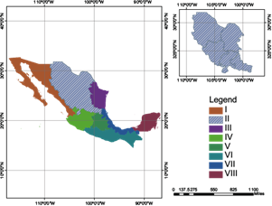
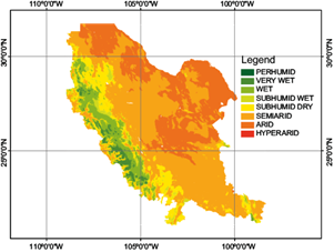
Eight economic regions of Mexico are described in reports by the National Commission for the Exploitation and Use of Biodiversity (Bassols, 1985; CONABIO, 2010). Each region can include more than one state that share characteristics of the biophysical environment and with common economic activities in the primary, secondary, and tertiary sectors. In the present work, region II is considered given its current characteristics as dry climates and limiting surface of water distribution, conditions that make it especially vulnerable to climate change from the point of view of drought (CONAGUA, 2021). Region II (Figure 1) covers the states of Chihuahua, Coahuila, Durango, San Luis Potosí and Zacatecas and it is located between 110 º 0 ‘0’ and 95 º 0 ‘0’ west longitude and 35 º 0 ‘0’ and 30 º 0 ‘0’ north latitude.
3. Materials and methods
Precipitation and temperature data were obtained from stations grouped in the Rapid Climate Information Extractor (ERIC) of the National Institute of Water Technology (IMTA) version III (IMTA, 2010). Data quality of many climatological stations is not good, with large gaps of missing data due to little maintenance and even permanent deactivation. Only 496 stations with 80% or more viable information were considered. The analyzed variables were maximum temperature (Tmax) and minimum temperature (Tmin) for the period 1970-2000. Precipitation values were obtained from the Informatics Unit for Atmospheric and Environmental Sciences (UNIATMOS) of the National Autonomous University of Mexico from 1950 to 2000 (UNAM, 2017).
Additional information was obtained from cartography of climate change models, scenarios of climatology (Hijmans, et al., 2005), climate global models, and emission scenarios of the Intergovernmental Panel on Climate Change (IPCC) that were processed and interpolated for Mexico and Central America, based on the Model for the Assessment of Greenhouse-gas Inducted Climate Change - MAGICC (UCAR, 2005).
3.1 Geostatistical analysis
The concept of spatial autocorrelation is supported by Tobler’s principle, which states that in a geographic space everything is related and the closest areas are more related (Tobler, 1970). Spatial autocorrelation helps to understand the degree of similitude of one object with another (ESRI, 2019). In general, there is spatial autocorrelation (SA) whenever there is a pattern in the behavior of the variable according to the geographical location of the data.
Geostatistical techniques require second-order stationarity data, that is, at least the variance must be the same in different sub-regions. The lack of stationarity is commonly linked to anomalies in space, or to the existence of a trend or spatial gradient whose dimension is greater than the study region (Cressie, 1993). Stationarity can be a problem when interpolating points in space, but it does not justify abandoning geostatistics in favor of other interpolation techniques such as inverse distance weighted (IDW) since it is equally sensitive to lack of stationarity as described by Isaaks and Srivastava (1989).
3.2 Moran’s Global Index and G general of Getis-Ord
The global Moran Index (Moran, 1950) measures spatial autocorrelation based on locations and values of the entities simultaneously. Given a set of entities and an associated attribute, it evaluates whether the expressed pattern is clustered, sparse, or random (ESRI, 2019). The Moran index (I) for spatial autocorrelation is given by equation (1):
where, z
i
= (x
i
- x̅) is the deviation of an attribute or characteristic
from its mean; x
i
is an attribute value for characteristic i; w
i,j
is a spatial weight between feature i and
j, n is the total number of features, and
S
0
is the aggregate of all spatial weights which is computed as follows,
The Getis-Ord general statistic (G) (Getis and Ord, 1992) measures the concentration of high or low values in a given study region and is given by equation (2):
where x
i
and x
j
are attribute values for characteristics i and
j, w
i,j
is the spatial weight between characteristic i and
j, n is the number of characteristics in
the data set. The null hypothesis for the High / Low Clustering statistic
(General G) states, H0 : There is no spatial grouping of entity
values vs the alternate hypothesis H1: There is a spatial grouping of
entity values. The test statistic is based on the standardized Getis-Ord index
given by
3.3. Kriging method
Kriging is an advanced geostatistical procedure that generates an estimated surface from a set of scattered points with z-values. The Kriging tool performs an interactive investigation of the spatial behavior of the phenomenon represented by the z-values before selecting the best estimation method to generate an output surface. The kriging technique assumes that data are correlated in space. The kriging method is considered to be BLUE (Best Linear Unbiased Estimator) and is similar to Inverse Distance Weighted. The general equation is given by:
where: Z(S i ) is the value measured at location i; λ i is an unknown weight for the value measured at location i; s 0 is a location and n is the number of measured values.
In ordinary kriging, λ i , depends on a fitted model, the distance to the location, and the spatial relationships between the measured values around the location. The kriging interpolation method describes dependency rules with variograms and covariance functions (spatial autocorrelation). The kriging methodology assumes that data follow a Gaussian distribution, present stationarity, are spatially continuous, and the autocorrelation is known, only then, kriging is considered an optimal predictor (Gallardo, 2006). In this work, ordinary kriging was chosen due to the nature of the data, in addition, it offers the possibility of making different adjustments through pre-established models.
For realizations of a variable Z at points x i , i = 1,2,… n, say, Z (x 1 ), Z (x 2 ),… Z (x n ), we want to estimate Z (x 0 ), and there was no measurement at x 0 . In this circumstance, the ordinary kriging method estimates the variable as a linear combination of the n random variables as follows:
where the λ
i
represent weights of the original values Ẑ
(x
0
) is the best linear estimator because the weights are obtained in such a
way that they minimize the variance of the estimation error; other interpolation
methods such as inverse distances or polygonal do not guarantee minimum
estimation variance (Samper and Carrera,
1990). Weights are estimated by minimizing V
[Ẑ (x
0
) - Z(x
0
)] subject to
3.4 Aridity index
Temperature varies as a function of altitude; the empirical method developed by Fries et al. (2012) estimates temperature in mountainous regions, calculates the ranges of variation of the annual temperature at different elevations by a simple linear regression model:
where y i is the temperature (in ºC), x i is the elevation (in meters above the sea level), i = 1,…, n the number of data points, α is the intercept or temperature at sea level, while β is the temperature variation for each meter that increases the elevation, as in nature there is an inverse relationship between elevation and temperature, the value of β is negative, e i is the random error, we assume e i ~ NIID (0, σ e 2 ), where “NIID” stands for Normal Independent and Identically distributed and σ e 2 is the variance associated to the errors. The elevation was estimated with models of geographical elevation provided by the National Institute of Geography and Statistics (INEGI, 2020).
The mean annual temperature layer was obtained with ordinary kriging
interpolation; ranges of 1ºC were generated. The Climate Influence Areas (Gómez et al., 2008) were obtained by cross
correlating the cartography of mean annual temperature with the estimated annual
precipitation. Potential Evapotranspiration (E) was calculated
with Thornthwaite method as follows. First, the monthly heat index was
calculated from the monthly mean temperature (T
i
, º C), as
The monthly potential evapotranspiration (mm/month) for months of 30 days and 12 hours of sun (theoretical), E “uncorrected” was calculated also based on temperature data, as:
where a = 675(10-9) (I 3 ) - 771(10-7) (I 3 ) + 1792 (10-5)(I) + 0.49239 is a theoretical adjustment coefficient. Finally, the calculation of the corrected E for month i is obtained through equation 8,
where, N i is the maximum number of hours of sunshine in month i and d i is the number of days in month i. The Aridity Index (AI) is a qualitative characteristic of the climate, which makes it possible to measure the degree of sufficient or insufficient precipitation. The Aridity Index (AI) was established in in Mexico through the Official Gazette of the Federation, on 1 June 1995 to define an aridity classification based on the Precipitation (P) and Evapotranspiration (E) as AI=P/E (DOF, 1995). The AI allows the classification into eight categories: hyper-arid (< 0.051), arid (0.051-0.201), semi-arid (0.201-0.501), dry subhumid (0.501-0.651), humid subhumid (0.651-0.751), humid (0.751-1.251), very humid (1.251-2.5) and per humid (> 2.5).
3.5 Setting scenarios in the near and distant future
Climate change scenarios are representations of future climate, based on an internally coherent set of climatologic relationships, which are constructed to investigate the potential consequences of climate change. Scenarios were constructed by superimposing layers of annual mean temperature and precipitation; and then databases were generated for the potential evapotranspiration and the AI. The centroids were obtained with automatic tracing of isotherms and isohyets; finally, global climate models were used to project data for near future (2015-2039) and far future (2075-2099), considering two values (4.5 and 8.5) of the Representative Concentration Pathway (RCP).
4. Results and discussion
4.1 Global Moran Index and Getis Ord G
The z-score of the Moran Global Index and G Index of Getis Ord, constructed with a weighting matrix under the K-nearest neighbor’s method, were 3.7797 and 5.5738 respectively; in both cases there is less than 1% probability that the pattern is the result of a coincidence, so there is indeed a spatial autocorrelation grouped in clusters for the case of the calculated mean annual temperature.
4.2 Predicted temperature
Fries, et al. (2012) indicate that it is necessary to consider the altitudinal gradient to obtain a correct temperature layer once the interpolation has been carried out, so the fitted linear regression model was:
The residuals were distributed randomly and with a presumably normal histogram, so we can conclude that the model complies with the assumptions of normality and homoscedasticity. Once the linear regression model was fitted, the equation proposed by Fries, et al. (2012) was used to predict the temperature:
where, T month corresponds to the mean annual temperature in º C; Γ corresponds to the altitudinal gradient calculated in the regression model (β̂ = Γ = -0.0042); T Det corresponds to a reference altitude (in this case 2000 meters above the sea level, used in the kriging methodology); and Z est corresponds to the elevation of each weather station in meters above the sea level.
4.3 Data normality
The Kriging procedure uses transformations in case data do not comply with the normality assumption, but it is difficult to use transformed values since it will later be necessary to work with the precipitation variable. A Shapiro-Wilk test was performed to verify data normality, with the hypothesis H0: The population is normally distributed vs. H1: The population is not normally distributed. A test value W = 0.97707 was obtained, with a p-value < 1 × 10⁻⁵, so setting the significance of the test at α = 0.05, we conclude that the population does not come from a normal distribution and a type of transformation is required. To correct the problem of normality, a subdivision of the study region was proposed, considering the physiographic provinces proposed by CONABIO, (CONABIO 2001) as shown in Figure 2.
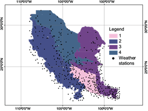
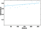
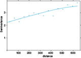
The physiographic provinces reduce extreme values and have homogeneous distributions. The Shapiro-Wilk goodness of fit test is shown in Table I, indicating that none of the sub-regions has normality problems. Once the assumptions were corroborated, the variograms of each physiographic province were obtained, as well as the adjustment of different models depending on the dispersion of Gamma values, as shown in Table II.
Table I Results of the Shapiro Wilk goodness of fit test.
| Sub Region | Shapiro Wilk’s W value | P-value for normality test |
| R1 | 0.9893 | 0.3298 |
| R2 | 0.9832 | 0.1325 |
| R3 | 0.9836 | 0.2689 |
| R4 | 0.9824 | 0.1659 |
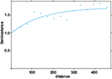
Table II Summary of adjustment of variograms, models marked in bold have the best fit and were selected.
| Physiographic Region | Model | SSR | Variogram and Fitted Model | Variogram attributes |
| R1 Center | Exponential Gaussian Spherical Circular | 63.21 60.62 60.16 60.44 |
|
Range:100 Psill: 0.9 Nugget:0.7 |
| R2 Western Sierra Madre | Exponential Gaussian Spherical | 38.97 326.57 36.64 |
|
Range:300 Psill: 4.0 Nugget:2.1 |
| R3 Eastern Sierra Madre | Exponential Gaussian Spherical Circular | 63.05 88.06 99.30 103.73 |
|
Range:200 Psill: 2.0 Nugget:1.0 |
| R4 North | Exponential Gaussian Spherical Circular | 95.43 18.39 18.61 18.11 |
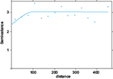
|
Range:100 Psill: 3.2 Nugget:2.1 |
4.4. Model validation
Model validation through different error indicators was carried out by two methodologies: Cross-validation and validation. Table III presents the summary of cross-validation, obtained through a random sample made up of 80% of the data, the variable temperature was estimated and validated with the stations not included in the sample. In general, values for mean, root mean square, standardized mean, root mean square standardized, and average standard error are small and some of them close to zero, therefore it can be concluded that the adjusted model seems to be correct.
Table III Summary of the cross-validation indicators, where R1, R2, R3 and R4 represent the previously defined sub regions.
| Topic | R1 | R2 | R3 | R4 |
| Sample | 117 | 142 | 173 | 98 |
| Mean | -0.0008 | -0.0157 | 0.0366 | 0.0245 |
| Root Mean Square (RMS) | 0.905 | 1.5362 | 0.0258 | 1.2813 |
| Standardized mean | -0.0010 | -0.0082 | 0.0209 | 0.0174 |
| RMS Standardized | 1.0858 | 1.0823 | 0.9856 | 0.8987 |
| Average Standard Error | 0.8319 | 1.3954 | 1.1772 | 1.4239 |
| Regression function | -0.006*x + 17.17 | -0.52 * x + 8.70 | 0.30 * x + 11.51 | 0.54 * x + 7.43 |
For the validation methodology, the data were divided into 2 subsets: a training set and a test set, the subsets are large enough to be representative and to generate statistically significant results. Again the estimations for average error, root mean square, and average standard error are close to zero, which indicates a good fit (Table IV). Once the validation of the models is completed, the temperatures are interpolated and the altitude gradient is adjusted.
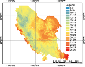
4.5 Isotherms
Sub-region R1, mainly presents temperatures between 14 ºC and 19 ºC, with some surfaces between 8 ºC and 10 ºC in the elevated regions, as well as temperatures of 22 ºC to 24 ºC in the northwest. For sub-region R2, there are low average temperatures throughout the summit of the western Sierra Madre with temperatures ranging between 8 ºC and 10 ºC, with the highest temperatures also occurring towards the east of the mountain, ranging between 24 and 26 º C. In sub-region R3, the highest temperatures are obtained in the southeast, coinciding with the warmest region of the state of San Luis Potosí, with average temperatures of 25 ºC to 26 ºC, as well as the coldest in the center with isotherms of 9 ºC to 10 º C. In sub-region R4, temperatures are generally observed ranging between 16 ºC and 18 ºC with the warmest surfaces to the east with temperatures ranging between 20 ºC and 23 º C (Fig. 3).
4.6 Precipitation
The total annual precipitation was obtained using map algebra
where i corresponds to the i-month evaluated. The result, reclassified to every 100 mm of rainfall, is presented in Figure 4. Twenty-one classes of precipitation were obtained, the most intense colors of blue being the regions with the highest rainfall.
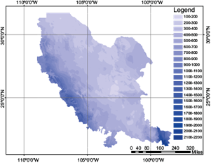
The precipitation is distributed as expected, the most humid regions are those corresponding to the windward part of the western Sierra Madre and the southern part of the state of San Luis Potosí. On the other hand, the regions with less precipitation correspond to the leeward part of both the western and eastern Sierra Madre, coinciding with the theory of Gómez et al. (2008).
4.7 Aridity index of base scenario
Monthly databases of climatic variables were generated for each CIA. Centroids of each polygon were obtained using geometric methods. The aridity index was calculated with estimations of annual mean temperature (Tmed), potential evapotranspiration (E), and precipitation (P). The baseline scenario was built with climate data from the 1970-2000 period. The data for the period 2000-2020 were not used because it shows a considerable decrease in quality in most of the stations considered. The calculated aridity baseline scenario is presented in Figure 5. The percentages for each classification were as follows: hyper-arid (0%), arid (1%), semi-arid (54%), dry sub-humid (15%), humid sub-humid (9%), humid (15%), very humid (6%) and per humid (0%). The baseline scenario for region 2 presents a predominance of a semi-arid climate with more than half of the surface region (in km2), the percentages of Per-humid and Hyper-arid climates are close to 0%. The highest concentration of humid regions is concentrated in the western highlands, more specifically in the windward region, and the driest regions are in the north-central region.
4.8 Global climate models
Table V and Figure 6 show the estimates of four global climate models considering two Representative Concentration Pathway (RCP) and two horizons (H1: 2015-2039 and H2: 2075-2099), in general, there is a transition from left to right, from humid classes to arid classes, the most optimistic scenario is CRNMCM5 where the “hyperarid” class is not reached and in the worst scenario, the closest horizon only occupies 6245.40 km2 of the “arid” class. The most pessimistic models are MPI-ESP and GFDL-CH3, since in both cases the “hyperarid” class is reached with 5639.26 km2 (0.9%) and 5621.52 km2 (0.9%) respectively. The class “perhumid” represented by just 1 km2 only exists in the base scenario and is extinguished in the rest of the scenarios. A model that is neither very pessimistic nor very extreme is HADGEM 2.0, which predicts an “arid” surface of 349325.99 km2 (53.8%) without reaching the “hyperarid” class.
Table V Results of estimates in percentage for different horizons in eight climate classes. Four models are presented.
| Classification | ||||||||||
| Model | RCP | H | Per humid | Very wed | Wed | Sub humid Wed | Sub humid Dry | Semi arid | Arid | Hyper arid |
| base scenario | - | 0 | 0.0% | 6.3% | 14.6% | 9.5% | 15.1% | 53.5% | 1.0% | 0.0% |
| HADGEM 2.0 | 4.5 | 1 | 0.0% | 4.8% | 14.1% | 2.0% | 13.5% | 64.7% | 1.0% | 0.0% |
| 2 | 0.0% | 2.8% | 15.6% | 2.3% | 5.1% | 73.1% | 1.0% | 0.0% | ||
| 8.5 | 1 | 0.0% | 7.6% | 12.9% | 3.4% | 13.7% | 61.5% | 1.0% | 0.0% | |
| 2 | 0.0% | 1.9% | 7.0% | 1.0% | 2.1% | 34.3% | 53.8% | 0.0% | ||
| CRNMCM5 | 4.5 | 1 | 0.0% | 9.9% | 12.6% | 6.4% | 9.1% | 61.1% | 0.9% | 0.0% |
| 2 | 0.0% | 3.6% | 16.4% | 1.1% | 11.3% | 66.7% | 1.0% | 0.0% | ||
| 8.5 | 1 | 0.0% | 9.6% | 11.4% | 4.6% | 12.6% | 60.9% | 0.9% | 0.0% | |
| 2 | 0.0% | 2.8% | 7.3% | 10.5% | 8.8% | 69.6% | 1.0% | 0.0% | ||
| GFDL-CH3 | 4.5 | 1 | 0.0% | 8.8% | 15.4% | 5.6% | 8.3% | 61.1% | 0.9% | 0.0% |
| 2 | 0.0% | 8.6% | 15.3% | 5.0% | 9.1% | 61.2% | 0.9% | 0.0% | ||
| 8.5 | 1 | 0.0% | 3.0% | 15.4% | 1.1% | 5.8% | 72.9% | 1.7% | 0.0% | |
| 2 | 0.0% | 2.8% | 5.6% | 8.8% | 6.6% | 20.9% | 54.4% | 0.9% | ||
| MPI-ESP | 4.5 | 1 | 0.0% | 7.3% | 12.9% | 2.6% | 9.7% | 66.5% | 1.0% | 0.0% |
| 2 | 0.0% | 3.5% | 7.0% | 10.4% | 9.9% | 68.3% | 1.0% | 0.0% | ||
| 8.5 | 1 | 0.0% | 3.6% | 16.8% | 2.4% | 9.1% | 67.2% | 0.9% | 0.0% | |
| 2 | 0.0% | 1.9% | 7.9% | 0.3% | 10.5% | 24.4% | 54.2% | 0.9% | ||
H: Horizons, 0: 1970-2000; 1: 2015-2039; 2: 2075-2099.
RCP: Representative Concentration Pathway.
HADGEM2.0: Met Office Hadley Centre (MOHC) (United Kingdom model).
CRHMCM5: Centre National de Recherches Météorologiques (French model).
GFDL-CH3: Geophysical Fluid Dynamics Laboratory (USA model).
MPI-ESP: Max Planck Institute for Meteorology (Germany model).
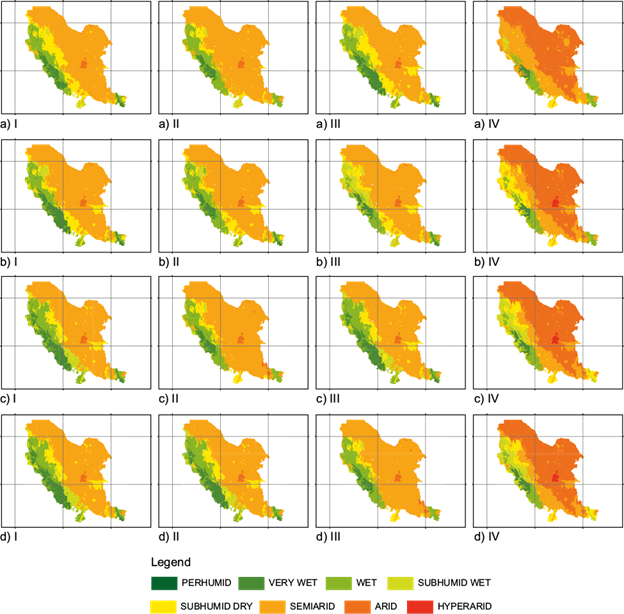
Fig. 6 Mapping of aridity evolution scenarios for models: a) HADGEM2.0; b) MIP-ESP; c) CRNMCM5; d) GFDL-CM3; I: RCP=4.5, Horizon 2015-2039; II: RCP=4.5, Horizon 2075-2099; III: RCP=8.5, Horizon 2015-2039; IV: RCP=8.5, Horizon 2075-2099.
In summary, the results indicate that all the assumptions of the Kriging model were fulfilled and, therefore, the best unbiased linear estimator was developed. The validation model showed that estimates were correct. A base aridity index and projections from global climate models were obtained for near and far futures. Such projections are useful to make decisions in the present and change the projected trend. All the global climate models predict an increase in aridity for the far future, and RCP = 8.5, so we should take action to avoid large RCP levels. The information generated in this study has technical foundations.
For future research, the study can be extended to develop projections for all regions of Mexico. Having reliable information helps us make the best decisions and, in terms of climate, it allows us to reduce climate change effects.
5. Final remarks
The availability of climate information in Mexico is severely affected by different factors, such as meteorological stations with no maintenance and less than 70% of the data. The aridity in regions where land has severe degradation problems can lead to a loss of productive capacity practically irreversible. The use of geostatistical interpolation methodologies for unsampled points is very useful to model the behavior of different climatic variables. Temperature and precipitation detailed maps were obtained for economic region II of Mexico. Different scenarios were predicted with global climate models. Results show adverse scenarios: in the best prediction, aridity will strongly weaken the humid ecosystems, and in the worst scenario hyper-arid climates will appear, practically inhospitable for many of the species with limited environmental resilience that today inhabit these regions. It is urgent to carry out specialized studies of territorial order, natural resources management, regeneration, and adaptation work for the regions where ecosystems are most vulnerable. Some proposals that can be highlighted are: well-managed reforestation plans, constant cooperation with multilateral organizations, transition towards clean and renewable energies, reducing emissions into the atmosphere, and reducing the potential of the highest Representative Concentration Pathways.
Although Mexico does not have an atmospheric circulation model, some efforts have been made to represent the country’s environmental conditions, and this study, supported by geostatistics, is one of them.

