


 nueva página del texto (beta)
 Inglés (pdf)
 Artículo en XML
 Referencias del artículo
 Enviar artículo por email
 Citado por SciELO
  Similares en
SciELO
Similares en
SciELO 
 Permalink
1. Introduction
The industrial revolution changed dramatically the planet’s atmospheric composition bringing air pollution and making it one of the biggest ongoing threats facing global public health. It is estimated that ~ 90% of the world’s population lives in areas where levels of air pollution are above limits deemed safe for human health (WHO, 2018). Worldwide, these levels are influenced by pressures for economic development (combustion processes for energy generation using technologies not internationally recommended) and, regionally, by each area’s topography and climate (Parra et al., 2009). This last factor, climate, acts from large to small scales, modulating emissions by increasing or decreasing them. The nature of emissions depends on their source and can be primary air pollutants (emitted directly into the air from a source) with direct impacts, or precursors for secondary air pollutants formed through reactions in the atmosphere (often in the presence of sunlight) such as oxides of nitrogen (Bimbaitė and Girgždienė, 2007; Schnitzhofer et al., 2008).
There are many chemical species of nitrogen oxides (NOx), but the air pollutant of most interest is nitrogen dioxide (NO2), not only because of its effects on human health but also because (a) it absorbs visible solar radiation and contributes to impaired atmospheric visibility; (b) as an absorber of visible radiation it can have a potential direct role in global climate change if its concentrations become high enough; (c) it is, along with nitric oxide (NO), a chief regulator of the oxidizing capacity of the troposphere by controlling the build-up and fate of radical species, including hydroxyl radicals, and (d) it plays a key role in atmospheric chemistry related to ozone formation and destruction, this being the main vector to absorption of ultraviolet radiation reaching the planet’s surface, whether in polluted or unpolluted atmospheres (WHO, 2000). As a significant contributor to air pollution, NO2 is released into the atmosphere from both natural and anthropogenic sources, being the major ones fossil fuel combustion, biomass burning, lightning, and ammonia oxidation. It is estimated that the lifetime of NO2 in the atmosphere varies from 6 h in summer to 18-24 h in winter (Seinfeld and Pandis, 1998; Bond et al., 2001; Beirle et al., 2003; Zhang et al., 2003). Its concentration level is influenced by complex variables such as wind, temperature, burning material, besides policies and other anthropogenic factors of each city (e.g., urban areas) (Liu et al., 2016; Wang and Su, 2020).
The growing trend in the emission of atmospheric nitrogen dioxide (NO2) has been a major concern around the world, the developing countries being at larger risk owing to fewer resources and socioeconomic vulnerability (Munzi et al., 2009). Traditionally, this trace gas is measured through a network of monitoring stations in the ground, but such an extensive network may not exist in all areas of interest and particularly in lower-income countries. An alternative approach to overcome these limitations is to use satellite data, which provide spatiotemporal data from regional to global scales under widely different atmospheric conditions and offer expeditious, accurate information about changes in air quality and their human impacts (Bais et al., 2007; Liu et al., 2016; Mostafa et al., 2021).
In South America, studies on air pollution are limited to a few cities, because air quality monitoring stations tend to be expensive, and not all air pollutants are monitored (Réquia et al., 2015; Fajersztajn et al., 2017; Silva et al., 2020). An example of the lack of an extensive network for environmental monitoring is the state of Rio Grande do Sul, located in south Brazil, with only nine stations within its borders. Compared to other regions of the country, it is exposed to higher levels of ultraviolet radiation for being closer to the Antarctic ozone hole (Kirchhoff et al., 2000; Guarnieri et al., 2004), and is strongly influenced by transient meteorological systems (cold and hot fronts), isentropic transport (between the tropical stratosphere reservoir, polar vortex, middle-latitude) and exchange processes (between upper-lower stratosphere) (Reboita et al., 2010; Bittencourt et al., 2019).
Recently, spaceborne observations were combined with statistical methods to produce spatiotemporal predictions on NO2 concentrations, supplementing existing ground-based stations and providing coverage where ground-based data are unavailable (Hoek et al., 2015; Larkin et al., 2017; Qin et al., 2020). These predictions are based on machine learning models ranging from linear regression models to non-linear, being the latter the ones that perform better since they consider that there is a non-linear relationship between predictor variables and dependent variables (Zhan et al., 2018a). Predictive variables of models for air pollutants usually include satellite data, meteorology, population density, elevation, and land-use type variables (Zhan et al., 2018b; Pan et al., 2021).
Random Forest (RF) is a non-linear model simple in structure, requires less computational resources, and has strong interpretation capabilities. Besides giving importance weights for each of the included variables to select the model predictors, it is also less prone to overfitting and less sensitive to outliers (Pan et al., 2021). Many of the NO2 studies based on this model have focused on short and long-term spatiotemporal changes (Hoek et al., 2015; Araki et al., 2018; Zhan et al., 2018a, b; Kamińska, 2019; Zhu et al., 2019; Qin et al., 2020), showing good prediction performance, with cross-validation R2 from 0.69 to 0.84. In addition, models in such studies exhibit higher accuracies when the dataset integrates temporal and spatial information.
Given that the existing environmental monitoring stations in Rio Grande do Sul are sparse and unevenly distributed, the objective of this study is to reconstruct the long-term spatiotemporal environmental NO2 concentrations from 2006 to 2019 across the state, through the RF machine learning model, using as input parameters data retrieved from the Ozone Monitoring Instrument (OMI) sensor aboard Aura satellite, besides meteorological covariates and ancillary data.
2. Material and methods
2.1 Study area
Rio Grande do Sul is the Brazilian southernmost state, having international borders with Argentina to the west and Uruguay to the south (Fig. 1). Its area is 281 707 km², and with more than 11.5 million inhabitants it is the fifth most populated state in the country; about 85% of its population lives in urban areas (Fig. 2). The metropolitan area of its capital, Porto Alegre, concentrates an important fraction of the state’s population and economic activities. Regarding the consumption of fossil fuels, the state has about 7.5 million vehicles (IBGE, 2021). The region has a humid subtropical climate with a large seasonal variation with hot summers and well-defined, cold winters. Mean temperatures vary from 15 to 18 ºC, with lows of as much as -10 ºC (June and July) and highs going up to 40 ºC (December to March) (Livi, 2002). The surface elevation ranges from sea level up to 1400 m, with the highest points northeast of the state (Fig. 2).
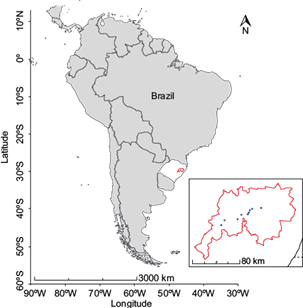
Fig. 1 Map with Rio Grande do Sul’s (Brazil) location (in white) and its metropolitan area (red contour) and the positions of NO2 monitoring sites (blue points).

Fig. 2 Topographic and demographic representations of Rio Grande do Sul, Brazil. Elevation (left), urbanization (right) (COREDES, 2010).
2.2 Data set
2.2.1 Ground-level NO 2 data
The ground-level NO2 data was acquired by nine monitoring sites (Fig. 1) managed by the Fundação Estadual de Proteção Ambiental (the state’s Environmental Protection Foundation, FEPAM), measured hourly by the chemiluminescence method from 2006 to 2019, with the occurrence of some discontinuous periods (FEPAM, 2021). For this research, we integrated the hourly average concentrations to daily values for all stations, and then all data were interpolated to a 0.25º × 0.25º grid. This spatial resolution was the standard in this study, and 420 such cells were necessary to cover the state. After this pre-processing, a total of 2229 daily measurements of ground-level NO2 were used to develop to model. This number represents 43.5% of the time series of 14 years if data were acquired every day during the studied period.
2.2.2 Satellite NO 2 data
The orbital data used in this study came from the OMI sensor onboard the Aura satellite. This instrument is equipped with a spectrometer pointed to the nadir which measures the ultraviolet light (264-504 nm) coming from the Sun and back-scattered by the atmosphere. The Differential Optical Absorption Spectroscopy (DOAS) algorithm was developed to derive NO2 (product OMNO2d) (Krotkov et al., 2006). The data provided in this product are expressed in molecules cm-2 units daily at 0.25º × 0.25º (latitude/longitude) spatial resolution, these column densities being adequate to track spatial patterns for ground-level NO2. Therefore, it is unnecessary to convert vertical column density to ambient concentrations in the input model (Bechle et al., 2015). These data are represented in a time series of 14 years (2006-2019), with 5092 daily images (99% of the series) acquired from the data provider GES-DISC (NASA, 2021a).
2.2.3 Meteorological data
The data of meteorological covariates were acquired from the Modern-Era Retrospective analysis for Research and Applications (MERRA-2) produced by the NASA Global Modeling and Assimilation Office (GMAO), which provides a global atmospheric reanalysis beginning in 1980. These data were initially produced on a 0.5º × 0.666º global grid and were re-gridded by the POWER project to the 0.5º × 0.5º (latitude/longitude) bilinear interpolated spatial grid with daily resolution. The daily meteorological conditions used in the model include surface temperature, wind speed, humidity, surface pressure, all variables to 2 m (Rienecker et al., 2011). This data are represented in a time series of 14 years (2006-2019) with 5113 images for each variable with daily measurements (100% of the series) acquired from the data provider POWER (NASA, 2021b).
2.2.4 Ancillary data
To support our model, data on elevation were included on the form of 90 m vertical resolution measurements collected by the Shuttle Radar Topography Mission (STRM) and acquired from the Federal University of Rio Grande do Sul (UFRGS, 2021), from which a mean elevation 0.25º × 0.25º grid was compiled.
Information on the erythemal daily dose and ozone were also added, provided by satellite OMI through product OMUVBG in J m-2 units with a daily spatial resolution of 0.25º × 0.25º (latitude/longitude). Daily data form the product OMTO3d (ozone total column density) were also included, but with a 1.0º × 1.0º (latitude/longitude) spatial resolution in Dobson units (where 1 DU = 2.7 × 10¹⁸ molecules O3 cm-3) (Levelt et al., 2006; Tanskanen et al., 2006). These data are represented in a time series of 14 years (2006-2019) with 5092 daily images (99% of the series), acquired from the data provider GES-DISC (NASA, 2021a).
2.3 Statistical model
Predicting NO2 concentration with sufficient spatial and temporal resolution and accuracy is not a simple task. Although satellite data can contribute to this problem, they are usually limited to a single measurement per day, and their units in vertical column density are difficult to compare with ground data (Liu et al., 2021). Nevertheless, there is a growing interest in combining ground-based data and satellite observations to produce information comparable with measurements at surface level (Lu et al., 2020).
Modeling concentrations, like those of NO2 presently in focus, can be achieved through a diversity of techniques, among which we can mention the Gradient Boosting Decision Tree (GBTD) and the XGBoost algorithms, besides support vector machine (SVM) supervised learning algorithms. For this study, modeling using the RF technique was chosen due to its potential to direct implementation and for its robustness, being less prone to overfitting and less sensitive to outliers (Breiman, 2001). Therefore, it constitutes a viable option to be applied to complex atmospheric processes, which provides a spatiotemporal estimate of air pollutants by using a simple regression model (Qin et al., 2020; Chan et al., 2021). The RF regression model consists of a collection of regression trees trained by bootstrap samples that splits each node in the regression tree according to the best of a subset of randomly chosen predictors (Liaw and Wiener, 2002). Each tree is a regression function on its own, and the final output is the average of the individual tree outputs. In this study, from the collected dataset of ground-level NO2 concentrations and various predictors such as satellite NO2 retrievals and meteorological variables (temperature, wind speed, relative humidity, and atmospheric pressure), plus the ancillary data, ground NO2 concentrations were simulated with the following expression:
where j is the cell and i is the day.
This regression model was applied in three phases:
Training set, where we used 70% of the database with the ability to predict concentrations observed in monitoring sites, based on a set of predictors. At the end of this phase the relative importance of the predictors is directly provided by the RF model.
Performance, where, according to our objective of estimating ground-level NO2 concentrations over places with no monitoring stations and from limited input data, we applied two validation methods: 10-fold cross-validation (over the training set), which is a re-sampling procedure used to evaluate if our model is under-fitting/over-fitting; and test set validation (with 30% of the database), used to the evaluation of the final model fit on the training dataset, with an assessment of the discrepancies between predictions and observations of the monitoring sites. These comparisons were summarized in terms of R2 (percentage of explained variance), root mean square error (RMSE), and mean absolute error (MAE). The two latter metrics explain the differences between predicted and true values; the smaller the RMSE and MAE, the smaller the error between these two.
Generalization, which estimates the concentrations in the cells where no ground-level observations were available (Liaw and Wiener, 2002; Zhu et al., 2019; Gariazzo et al., 2020; Dou et al., 2021).
2.4. Analysis
The machine learning method used to estimate ground-level NO2 concentrations in this study area is summarized in Figure 3, which shows collected and standardized multi-source data used to obtain the desired dataset with uniform spatial-temporal resolution (0.25º × 0.25º [latitude/longitude], daily resolution). The Pearson correlation coefficient was calculated for all predictors and ground observation data before running the model to evaluate the effect of these parameters.

Fig. 3 Flow diagram of this study: daily ground-level NO2 concentrations based on the Random Forest model.
To predict in all 420 cells through Random Forest, we used the R caret package (Kuhn, 2008; Wright y Ziegler, 2017), which is an interface that unifies several functions from different packages under the same framework, facilitating all the stages of preprocessing, training, optimization, and validation of predictive models. For the Random Forest function, the user can only adjust two parameters (ntrees and mtry), considered by developers to have the greatest effect on the accuracy of the model. Accordingly, we adjusted the number of trees (ntrees) and, to avoid a suboptimal number of variables (mtry), we indicated a random search on the training dataset for tuning. This random search was done by 10-fold cross-validation (random sampling method), which involved dividing the dataset into folds of equal sizes, performing the analysis on one subset (training), and validating on the other subset (validation). To reduce variability, multiple iterations of cross-validation were performed using different partitions, the results being combined (e.g. averaged) to give an estimate of the model tuning and performance. Based on these cross-validation results, we finally set for the final model the ntree to 500 and the mtry to 10. All maps have been produced with the R statistical software, version 4.0.5 (http://R-project.org).
The evaluation of the long-term trend (2006 to 2019) of ground-level NO2 concentrations was made using the predicted values, calculating the cell averages for all 420 cells of the study area, for the whole period (historical series), as well as for month and season. The averages were calculated using the daily values for each of these periods, as follows:
where Ave i is the average of the variable in each cell for the respective period; start date and end date correspond to the first and last date of each period; n is the number of days in the period.
The total average concentrations of ground-level NO2 were evaluated by summarizing average concentrations across all cells that represent the State throughout each period.
3. Results and discussion
3.1 Model performance assessment
Relationships between ground-level NO2 and each independent attribute are shown in Figure 4. The variables with the strongest correlation were: Year (r = -0.44), Satellite NO2 (r = 0.24), Erythemal daily dose (r = -0.21), and Wind speed (r = -0.17). It can be noted that the dependent variable is influenced by interannual variations, dispersion, and photochemistry; however, variables with lower correlations also play a role in the model construction, as shown in Figure 5, which gives a perception on the contribution of variables to the final model. The categorical variable Year is the most important with a relative value of 1, followed by Elevation (0.5), Wind speed (0.26), Julian day (0.26), Erythemal daily dose (0.24), and sixth but not least, Satellite NO2 (0.20). The remaining variables are ranked as less important. It has been reported that the satellite NO2 (vertical column density) variable can be ranked as one of the most important in most models that use machine learning techniques to predict NO2 (Araki et al., 2018; Zhu et al., 2019; Qin et al., 2020; Dou et al., 2021; Chan et al., 2021), but some of these studies have shown that this importance varies between geographical areas and it may turn into one of the least important variables, contributing in some cases with only 1% of the prediction. This variation can occur for two reasons, the first one being due to the spatial resolution of this product since variations of NO2 were averaged within each cell. The second reason is that the sensitivity of the OMI sensor and of any satellite-based NO2 measurement increases with altitude, implying that measurements at ground-level are less sensitive due to scattering of radiation at the surface and through the atmosphere (Lu et al., 2020; Penn and Holloway, 2020; Di et al., 2020).


Fig. 5 Relative importance of predictor variables in the Random Forest model. Variables are listed in order of importance from top to bottom. The horizontal axis represents the measure of importance.
Results expressing the model performance are presented in Figure 6 as a scatter plot, where the 10-fold cross-validation method yielded R2 = 0.68, RMSE = 6.43, and MAE = 4.37. The test set validation method used to evaluate the model’s performance yielded R2 = 0.70, indicating the ability of the model to predict unknown data. The model metrics presently reported express a performance similar to those obtained by Qin et al. (2020) and Dou et al. (2021)1, who also adopted 0.25º × 0.25º spatial resolutions to estimate ground-level NO2. We note, however, that in regression models the adopted spatial resolution of the predictors will depend on the objectives pursued, and for many applications data a finer (≤ 1 km2) spatial resolution is necessary to capture environmental variability that can be partly lost at lower resolutions (Hijmans et al., 2005).

Fig. 6 Scatter plot result for the Random Forest model 10-fold cross-validation. The red dash line is the 1:1 reference line, the blue solid line is the trend line. The color bar indicates the number of data points.
In models like the one presently developed it has been shown that analysis of the spatiotemporal distribution of a variable with spatial dependencies can suffer from a misinterpretation of certain predictor variables (e.g., coordinates and elevation), an issue that has been reported as a disadvantage for flexible algorithms (e.g., Random Forest) when predicting beyond the location of the training data (Meyer et al., 2019). In such cases, the predictive performance becomes more sensitive to the sample sizes or absolute values of dependent variables (Zhan et al., 2018a; Li et al., 2020). In the case presently investigated, Elevation is one of the most important variables to the final model, which was built from data by nine ground monitoring stations with elevations between 20 to 85 m, while the whole study area displays elevations between 0 and 1400 m; this fact possibly represents a limitation to this analysis, on an extent that has to be evaluated by further studies. However, an additional assessment of this model performance, in the form of a comparison between observed and predicted ground concentrations for the area covered by the nine monitoring stations, suggests that deviations due to elevation would have low weight, since, as it is presented in Figure 7a, the modeled concentrations closely follow the measurements over the studied period.

3.2 Spatial and temporal distribution of ground-level estimated NO 2
Table I presents the total estimated ground-level NO2 concentrations over the entire state for the period 2006 to 2019. From the RF model, the predicted ground-level NO2 concentrations across Rio Grande do Sul for this period have a mean of 18.73 μg m-3, a minimum of 8.67 μg m-3, and a maximum of 24.94 μg m-3, with a standard deviation of 3.86 μg m-3. From Table I and Figure 7b it can also be noted that the total modeled NO2 concentrations over the entire state showed a decreasing trend from 2006 to 2019. This decreasing trend can be expressed by what we presently call the interannual variability, which is the difference between the mean NO2 for each year, minus the average for the whole period. Considering that 2006 has the highest mean concentrations, and 2017 the lowest, the interannual variability decreases almost steadily, going from as high as 36.37 μg m-3 in 2006 to as low as -11.20 μg m-3 in 2017. Considering that burning of biomass and fossil fuels is the main source of NO2, this decrease could be at least partly explained, for the fossil fuels, by federal regulations of 1997 reinforced in 2008, making mandatory the installation of catalytic converters in all cars; for biomass burning, fires in crops and grazing fields were outlawed in 1992 in the State, and the legislation were slowly, but steadily enforced since then. We note that in Rio Grande do Sul state, forest fires are virtually non-existent. A final remark concerning this trend is that similar declines in NO2 concentrations were observed in several countries, having as reference approximately the same periods (UBA, 2020; DEFRA, 2021; US-EPA, 2021), and for similar reasons.
Table I Historical modeled means of NO2 from 2006 to 2019 for Rio Grande do Sul state, Brazil.
| 2006 | 2007 | 2008 | 2009 | 2010 | 2011 | 2012 | 2013 | 2014 | 2015 | 2016 | 2017 | 2018 | 2019 | ||
| State | Min | 18.14 | 18.28 | 9.64 | 9.84 | 8.97 | 8.40 | 8.34 | 8.14 | 6.54 | 6.13 | 5.56 | 5.48 | 4.63 | 3.25 |
| Max | 65.92 | 50.64 | 31.28 | 28.38 | 23.42 | 19.88 | 17.42 | 17.27 | 16.49 | 15.84 | 14.64 | 20.07 | 14.28 | 13.61 | |
| Mean | 55.10 | 43.88 | 25.69 | 23.57 | 18.99 | 16.12 | 14.34 | 12.00 | 10.31 | 8.84 | 7.95 | 7.53 | 8.95 | 8.97 | |
| SD | 13.68 | 9.43 | 6.22 | 5.25 | 3.94 | 3.03 | 2.29 | 1.55 | 1.42 | 1.14 | 1.06 | 1.22 | 1.62 | 2.19 |
Figures 8, 9 and 10 show the spatial ground-level NO2 distribution across the state in different time scales. Figure 8 shows the spatial distribution averaged over the entire 2006 to 2019 period, and to better understand this distribution we linked the information on elevation and percentage of urbanized areas in the state (Fig. 2) with the predicted concentrations in Figure 8. About elevation, we noted a pattern between of NO2 concentrations with elevation: up to 100 m, concentrations are between 10-15 μg m-3; from 400-600 m, between 15-25 μg m-3; a decrease is observed between 600-800 m (15-20 μg m-3) and finally, from 800-1400 m the increase is continuous. It has been reported that, in general, higher altitudes show lower NO2 concentrations (Zhu et al., 2019; Chan et al., 2021), since in meteorological situations of inhibited wind transport/advection pollutants can accumulate in depressions (valleys and basins) (Giovannini et al., 2020). However, the atmospheric interactions with orography at different spatial scales influence the dispersion of atmospheric pollutants, being more complex in rough terrains. As a result, pollutants can be transported by orographic flows to mountainous areas, arriving to significant concentrations where they were not locally emitted. These constraints are reinforced by the fact, that, in Figure 8, higher NO2 concentrations coincide either with urbanized, industrialized zones (some of which are situated in areas with elevations of about 800 m or higher), or with areas of intensive agriculture (where fertilizers are sources of NO2, and diesel-powered machines are heavy NO2 producers); in some regions, both factors are summed up (Guo et al., 2020; Ai et al., 2021).
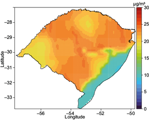
Fig. 8 Satellite-derived historical mean NO2 concentrations (μg/m3) throughout Rio Grande do Sul from 2006 to 2019.

Fig. 9 Satellite-derived monthly mean NO2 concentrations (μg m-3) throughout Rio Grande do Sul from 2006 to 2019.

Fig. 10 Satellite-derived season mean NO2 concentrations (μg m-3) throughout Rio Grande do Sul from 2006 to 2019.
NO2 concentrations are essentially a marker for combustion-related emissions and population, the latter having a direct relationship with urbanization levels. In this study, an inverse relationship was observed of the distribution of NO2 concentrations with urbanization levels, highlighting the highest concentrations in less urbanized areas < = 70%, with 15-20 μg m-3 averages. This apparently unexpected result is possibly due to the fact that some of the less urbanized areas are dominated by intensive agriculture, which become the major silent source of NOx pollution, and where soil microbes convert fertilizer to nitrogen oxides, emitting about as much gases as vehicles. The emissions of these biogenic sources are larger in areas with high N fertilizer applications (Oikawa et al., 2015; Almaraz et al., 2018). In Rio Grande do Sul, Mossmann Koch et al. (2018) also highlighted that even apparently uncontaminated sites, such as small rural cities with little urbanization and family farming as main economic activity, present higher or similar concentrations than urbanized and industrialized areas. In addition, combustion emissions in rural regions are dominated by biomass burning (e.g., human-initiated burning for crop preparation) (Bechle et al., 2011).
With respect to monthly and seasonal distributions (Figs. 9 and 10), these exhibit behavior similar to other studies, with lowest concentrations in January with a mean of 15.65 μg m-3 and standard deviation of 2.62 μg m-3 (Table II). In spring and summer concentrations assumed lower values, the latter with the lowest value (mean 16.75 μg m-3) (Table III). Highest concentrations were observed in May with a mean of 25.44 μg m-3 and standard deviation of 5.24 μg m-3 (Table II), while in fall and winter high concentrations were observed, the latter with a higher value (mean of 23.93 μg m-3) (Table III). In this context, due to its location, Rio Grande do Sul is under the action of a climatic complex whose action in spring and summer has the predominance of a tropical continental mass (a tropical Atlantic and a polar Atlantic mass), so that high humidity and high temperatures make the climatic conditions warmer, resulting in episodes of intense atmospheric convection and frequent precipitation which lead to the dispersion and wet deposition of NO2, reducing air pollution. Additionally, in summer, with longer sunshine durations along with higher temperatures and evaporation, hydroxide (OH) concentrations are boosted, leading to a lower lifetime of NO2, which becomes nitric acid (HNO3). In contrast, in autumn and winter, essentially under the control of equatorial Atlantic, tropical Atlantic, continental tropical, and polar masses, there is an intensification of the action of cold fronts in the state, enhancing cold weather and reducing humidity (less precipitation and higher atmospheric pressure) with respect to other seasons, conditions that are unfavorable for pollution dispersion (Rossato, 2011; Zhu et al., 2019; Qin et al., 2020; Dou et al., 2021).
Table II Monthly means of NO2 from 2006 to 2019 for Rio Grande do Sul state, Brazil.
| Jan. | Feb. | Mar. | Apr. | May. | Jun. | Jul. | Aug. | Sep. | Oct. | Nov. | Dec. | ||
| State | Min | 8.79 | 8.28 | 7.95 | 10.02 | 10.82 | 11.04 | 11.00 | 9.75 | 9.02 | 7.44 | 7.72 | 8.56 |
| Max | 19.79 | 20.47 | 23.78 | 28.23 | 31.03 | 31.14 | 29.50 | 27.72 | 26.94 | 24.26 | 22.35 | 23.43 | |
| Mean | 15.65 | 16.08 | 18.66 | 22.65 | 25.44 | 25.39 | 24.27 | 22.20 | 21.51 | 19.01 | 17.32 | 18.47 | |
| SD | 2.62 | 2.98 | 3.98 | 4.57 | 5.24 | 5.22 | 4.94 | 4.68 | 4.74 | 4.44 | 3.69 | 3.73 |
4. Conclusions
In this study, the use of Random Forest method, in combination with extensive data collection on multiple parameters from satellite and ground sources, was shown to be a valid tool for predicting NO2 ground level concentrations at low spatial and daily temporal resolutions in Rio Grande do Sul, Brazil. However, other modeling techniques are available, and their performance will be assessed in future studies.
The modeled NO2 seasonal variations at troposphere level displayed a higher concentration in winter, followed by autumn and spring, while summer had the lowest values during the 14 years covered by the study. In this context, such spatiotemporal trend is the combined effect of meteorological, geographical, and anthropogenic factors that, together, determine the increase or decrease of their concentrations.
Although the accuracy of modeled ground-level NO2 still needs to be improved, especially considering elevation variations, the spatial and temporal estimates presented here can allow the formulation, planning, and implementation of environmental policies considering present and future emission sources. In addition, we highlight the need for designing studies aimed at investigating both short-term and long-term air pollution, not only in major cities but also in suburban and rural areas.

