nueva página del texto (beta)
 Inglés (pdf)
 Artículo en XML
 Referencias del artículo
 Enviar artículo por email
 Citado por SciELO
  Similares en
SciELO
Similares en
SciELO 
 Permalink
1. Introduction
Air pollutants (gases and particles) are a matter of great interest due to their impacts on climate and public health (IPCC, 2014, 2021; Abbass et al., 2017; Soleimani et al., 2020). Although air pollutants are a very small fraction of the Earth’s atmospheric composition, they contribute to climate forcing and affect the hydrological cycle (Hinds, 1999; Ramanathan et al., 2001). Air pollutants play a critical role in the reproduction of biological organisms and in causing or enhancing diseases (Pöschl, 2005; Amsalu et al., 2019; Li et al., 2019; Peeples, 2020; Romano et al., 2020). Air pollutants originate from a variety of natural and man-made sources (Hidy, 2019). Particles may be divided into two categories: primary particles that are emitted directly into the atmosphere in liquid or solid form from burning of biomass and fossil fuel, volcanic eruptions, wind-forced suspension of mineral dust, sea salt and biological materials (Tomasi et al., 2017); and secondary particles that form by nucleation, condensation and reaction of gaseous precursors. Both primary and secondary particles are distributed in the atmosphere through turbulent mixing and wind transport (NASEM, 2016). Air pollutants, with a short life span of about a week in the troposphere, generally disperse from the source of origin and are highly variable spatio-temporally (Kedia and Ramachandran, 2009). In the troposphere, the diameter and mass concentration of air borne particles typically vary in range between 10-9-10-4 m and 1-100 µg m-3, respectively (Hinds, 1999; Raes et al., 2000; Pöschl, 2005).
To better understand the role of air pollutants in the tropospheric chemistry, a detailed characterization of air pollutants from in-situ and remotely sensed observations is needed (Kaufman et al., 1997). The air pollutants focused in this study include carbon monoxide (CO), sulphur dioxide (SO2), hydrogen sulfide (H2S), nitrogen oxides (NO2, NO, NOX), ozone (O3), and particulate matter (PM10). CO, SO2 and NO2 are hazardous gases produced by, for instance, fuel burning. H2S is also a toxic gas emitted into the atmosphere by organic material decomposition and fuel refining. Surface O3 has detrimental effects on public health, agriculture and the associated ecosystems; it is not directly released into the atmosphere, but is formed as a product of interaction between NOX and volatile organic compounds (VOCs) in the presence of sunlight. PM10 particles, having an aerodynamic diameter less than or equal to 10 μm, can be found in different shapes varying from irregular, platy, spherical, rod-like to angular. It is of great concern due to its adverse effects on humans and environment (Raizenne et al., 1996; Tawabini et al., 2017).
Investigation of spatio-temporal distributions of air pollutants, their cross-effect and the influence of meteorological variables such as atmospheric pressure, temperature, rainfall, relative humidity, wind speed and direction (PR, TC, RF, RH, WS, and WD, respectively) on air pollutant properties is essential for an understanding of climatology and spatio-temporal distribution characteristics of air pollutants (NASEM, 2016; Ordóñez et al., 2019; Rahman et al., 2019). Meteorological variables influence air quality not only on short term basis (daily and weekly) but also on long term basis, i.e., seasonally and annually (Zhang et al., 2018a).
Given that considerable challenges on the availability of air quality data remain in developing countries (Alvarado et al., 2019; Brauer et al., 2019; Pinder et al., 2019), it is not surprising that only a few studies have been carried out for the characterization of air pollutants in the region of Saudi Arabia: Hassan et al. (2013) monitored NO, NO2 and O3 in Jeddah city; Al-Jeelani (2014) investigated the diurnal and seasonal variations of surface O3 and its precursors, and SO2 in the atmosphere of Yanbu; Alghamdi et al. (2014) analyzed diurnal and seasonal variations of O3 and NOX concentrations in Jeddah city; Lihavainen et al. (2016, 2017) analyzed air pollutant concentrations in Hada Al Sham in western Saudi Arabia using single ground monitoring station data.
Dust events occur all year round in Saudi Arabia, with maximum intensity during spring and summer (Mayer, 1999; Yu et al., 2013; Maghrabi and Al-Dosari, 2016; Namdari et al., 2018). Dust storms are found to elevate PM10 concentration (Al-Hemoud et al., 2018). Relatively little attention has been given to cyclonic and anti-cyclonic extreme weather events in previous studies in relation to air pollutants. Weather events that encompass large spatio-temporal fluctuations in air pollutants play an important role in socio-economic life. As the study area is highly prone to dust events, this study also considers in some detail the detection of changes in air pollutant concentrations associated with extreme weather events (Tazeem, 2018).
Thus, this study focuses on understanding the spatio-temporal characteristics of extreme air pollutant events and its interdependency on meteorological variables. An added value of this study is to assess the relationship between air pollutants and meteorological variables using in-situ observations for an extended continuous period of 5 years (2008-2012); such a detailed study has not been previously done in the data-sparse region of Saudi Arabia.
2. Data and methodology
2.1 Data
2.1.1 Study area and ground-based data
Saudi Arabia is located in Southwest Asia and covers almost 80% of the Arabian Peninsula area (Vincent, 2008). It lies between 16-32º N latitude and 34-56º E longitude, and has one of the warmest and most arid climates of the world (Athar, 2014). There are no large inland water bodies except for the Red Sea bordering the west, whereas the Arabian Gulf borders east of Saudi Arabia, and Oman and Yemen to the south. Haqel is a relatively small city near the Red Sea, approximately 5 km away from the Jordanian border in northwest Saudi Arabia (Fig. 1). The region of Jeddah comprises three different geomorphological zones; the Red Sea and shoreline, the coastal plain, and low-lying coastal hills and pediments in the east.
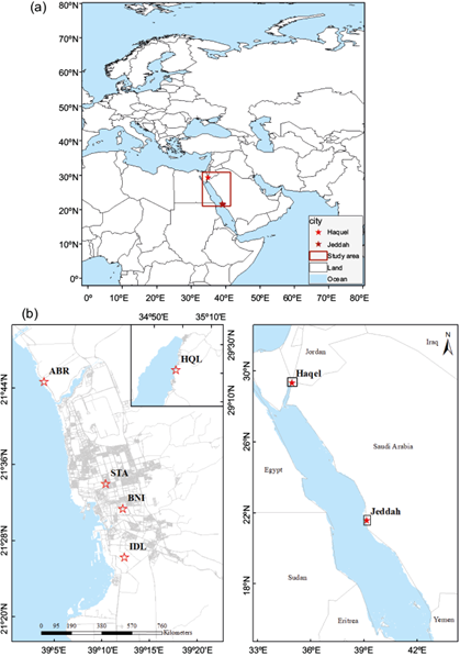
Fig. 1 (a) Map of the study area indicating location of the monitored sites and an averaging box encompassing all monitoring stations. (b) Location of the five monitoring stations for air pollutants and meteorological variables in Haqel and Jeddah, Saudi Arabia.
The data collected from five different ground-based stations for air pollutants includes CO, H2S, SO2, NO2, NO, NOX, O3 and PM10 and meteorological variables include RF, RH, PR, TC, WS and WD from January 2008 to October 2012, with an observation frequency of 15 min. Data was obtained from the Presidency of Meteorology and Environment, Jeddah, for five air quality monitoring stations, with four located in Jeddah: Abhur (ABR), Stadium (STA), Bani Malik (BNI) and Industrial area (IDL), and one located in Haqel (HQL). Table I displays the latitude/longitude, elevation and data availability period of the five air quality monitoring stations from which data was obtained.
Table I Details of air quality and meteorological variables monitoring stations, including latitude/longitude, elevation and start and end date of data availability.
| Station | Abbreviation | Latitude (N) | Longitude (E) | Elevation (m) | Start date | End date |
| Haqel | HQL | 29º21′18.62” | 34º57′39.98” | 12.19 | 01/01/08 | 13/10/12 |
| Abhur | ABR | 21º44′40.45” | 39º03′56.06” | 6.70 | 01/03/08 | 13/10/12 |
| Stadium | STA | 21º33′57.87” | 39º10′24.51” | 18.59 | 01/01/08 | 13/10/12 |
| Bani Malik | BNI | 21º31′22.95” | 39º12′11.14” | 18.28 | 01/01/09 | 13/10/12 |
| Industrial | IDL | 21º26′16.27” | 39º12′22.60” | 13.11 | 01/06/08 | 13/10/12 |
The ABR station is located at the sea bay near the east coast of the Red Sea, 30 km from Jeddah city. It is a tourist destination surrounded by a number of resorts, and thus contributes to both fixed and mobile sources of anthropogenic emissions. The STA station is located in the middle of the residential area of Jeddah city, and thus contributes dominantly to fixed sources of anthropogenic emissions. The BNI station is located in a busy shopping area, in the sub-urban corner of the main city, and thus contributes to both types of anthropogenic emissions. The IDL station is located near Jeddah’s industrial city, and thus is a source of industrial pollutants (such as SO2). The HQL station is located in sub-urban area of Haqel city, and thus has less vehicular related emissions. It is a source of more anthropogenic surface O3 emissions.
2.1.2 Satellite and reanalysis-based data
In this study, remotely sensed aerosol optical depth (AOD) observations were utilized. They were obtained from the ozone monitoring instrument (OMI) at 442 nm. The remotely sensed data is also utilized to study the behavior of meteorological variables, including atmospheric infrared sounder-based geopotential height at 925 hPa (AIRS H 925 ). For some recent reviews and applications that use satellite data for assessing regional air quality see, e.g., Engel-Cox et al. (2004), Martin (2008), Kumar et al. (2018), Sowden et al. (2018), Ali et al. (2020), Stirnberg et al. (2020).
Furthermore, the 10 m average daily wind data was obtained from the National Centers for Environmental Prediction/National Center for Atmospheric Research (NCEP/NCAR), Boulder, CO, USA. This global gridded wind data is available at a horizontal resolution of 2.5º × 2.5º, separately for the u and v wind components (Kalnay et al., 1996).
2.2 Methodology
2.2.1 Quality control
Multiple quality control measures were performed on the data prior to analysis throughout the study period (Athar, 2014). Values greater than 3σ were checked for extreme events from a 5-year average. Monthly and yearly averages were computed with at least 70% availability of the data (Mora et al., 2017). The minimum (maximum) number of missing days for STA (HQL) were 9.28% (26.23%). The data was stratified at different time scales and whenever possible compared with the USA based Environmental Protection Agency (EPA) air quality standards.
An air quality index (AQI) is devised to help understand the air quality of an area. According to the USEPA, an AQI index of more than 100 indicates (a moderately) unhealthy air quality and correspond to a certain level of air pollutants, i.e., 10.35 mg m-3 of CO and 147 µg m-3 of O3 averaged over 8 h, 196.5 µg m-3 of SO2 averaged over 1 h, and 150 µg m-3 PM10 averaged over 24 h.
The percentiles computed for air pollutants were compared with the EPA based AQI values for CO, SO2, O3 and PM10 for the following three classes: low (0-50), moderate (51-150), and high (151-300). A comparison of the percentiles for four air pollutants (O3, CO, SO2 and PM10) with the AQI is presented via box whisker plots in Figure 2.
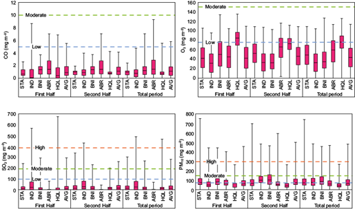
Fig. 2 Box whisker plots of 8-h averages of CO and O3 (upper row panels); 1-h averages of SO2 and 24-h averages of PM10 (lower row panels), at each station and their average, during the first and second halves, and the total time, of the study period (2008-2012). The horizontal dashed lines in each panel indicate USA-EPA air quality index levels.
2.2.2 Temporal variations
The data was temporally stratified on an hourly, daytime, nighttime, weekly, monthly, seasonal and annual basis. The seasonal variations were analyzed using March-May as spring of June-August as summer, November-October as autumn, and December-February as winter, whereas November-April are considered as the wet season and June-September as the dry season (Athar, 2015).
Computation of the weekend effect was also carried out to identify anthropogenic origins. In Saudi Arabia, weekdays are from Saturday to Thursday, with Friday as weekend. The weekend effect is thus considered as the difference between the weekend (Friday) and weekdays (Saturday-Thursday) values.
2.2.3 Percentile-based analysis
Percentiles are considered as an effective statistical measure for the analysis of trends because of their independency on skewness of data and on extreme values or outliers (Wilks, 2020). Percentile-based analysis is used to assess variation in low to high concentration scales (Iqbal and Athar, 2018). Data was divided into two half intervals to study percentile variability. Percentiles for each interval and the difference between the two halves was analyzed.
2.2.4 Extreme events
Modulations in air pollutant concentrations associated with cyclonic extreme events were noticed earlier in Riyadh, Saudi Arabia (Alharbi et al., 2013), as well as on larger scales, encompassing much of the Arabian Peninsula (Prakash et al., 2015). Climatologically, dust storm events occur dominantly in spring and summer in the Arabian Peninsula (Albaqami, 2019). Such extreme weather events were identified in the data and were compared with AOD measurements for validation over the study area.
The behavior of meteorological variables was also observed using AIRS H925 data. Wind data, obtained from the NCEP/NCAR reanalysis, was then used as visual aid to validate the presence of extreme weather events. The study aims to supplement trends tentatively presented in previous studies and to assess the relationship between air pollutants and meteorological extreme events.
2.2.5 Blocking events
Atmospheric anti-cyclonic blocking events occur when a high-pressure weather system persists for a number of days or weeks (for a recent discussion, see Woollings et al., 2018; Luo and Zhang, 2020). This persistence can lead to extreme weather conditions such as heat waves or cold spells and severe air pollution episodes due to air stagnation. In this study, blocking events recorded by the Global Climate Change Group of the University of Missouri (Colorado, USA) were analyzed and compared with ground and satellite-based observations to assess characteristics of blocking events and their association with high PM10, O3 and other air pollutant levels in the study region during the 5-year study period (2008-2012).
Blocking events with high PR centers at 30º to 50º E were analyzed in the study (Fig. 1). To diagnose the implications of these phenomena in the study area, blocking events from the catalog were checked for significant deviations from non-blocking periods using the Student t test for air pollutant concentrations and meteorological variables. Average measurements of AOD, O3, NO2, SO2 and CO vertical column for the study area during the blocking period were compared with blocking lifetime periods and with the length of non-blocking periods before and after blocking (nine days for short-span blocking event and 17 days for long-span blocking events) to assess the differences in daily means. Ground-based daily data of air pollutants and meteorological variables for all stations were also averaged and compared to identify statistical differences before, during and after the blocking period, if any (Table II).
Table II Dates of blocking events and their central longitude, including details of satellite based and in situ observations of air pollutants and meteorological variables. Statistically significant differences between before-during, during-after and before-after the blocking period are marked with vertical arrows next to the corresponding variables.
| Blocking dates | Longitude (ºE) | Satellite variables | In situ variables | ||
| Air pollutant | Meteorological variables | Air pollutant | Meteorological variables | ||
| 03/06/08-09/06/08 | 50 | - | - | - | TC (↓↑↓) WS (↑↓↑) |
| 11/06/08-19/06/08 | 50 | AOD (↓↑↓) O3 (↑↓↑) | - | - | WS (↑↓↓) |
| 15/07/08-24/07/08 | 40 | O3 (↑↓↑) | H500 (↓↑↓) | CO (↑↓↑) | - |
| 02/05/09-24/05/09 | 40 | AOD (↓↑↓) | H500 (↓↑↑) | NO2, NO, NOX, (↓↑↓) CO, O3 (↓↑↑) | PR, WS (↑↓↓) |
| 02/09/09-08/09/09 | 50 | O3 (↓↑↑) | - | NOX (↓↑↑) | - |
| 22/06/10-02/07/10 | 50 | AOD (↑↓↑) | - | - | PR (↓↑↓) |
| 20/07/11-27/07/11 | 50 | - | H1000 (↓↑↓) | NO, CO (↓↑↓) | RH (↑↓↑) |
| 17/08/11-24/08/11 | 30 | O3 (↓↑↓) | - | O3 (↑↓↑) SO2 (↓↑↓) | - |
| 08/09/11-21/09/11 | 50 | - | - | NO2, NOX (↓↑↓) | TC (↓↑↓) |
| 08/10/11-16/10/11 | 50 | - | - | O3 (↑↓↑) | WS (↑↓↑) |
| 06/05/12-23/05/12 | 30 | AOD (↑↓↑) | H500 (↓↑↑) | PM10 (↑↓↑) | TC (↓↑↑) |
| 27/05/12-07/06/12 | 30 | - | H1000 (↑↓↓) | SO2 (↑↓↓) | PR (↓↑↑) |
AOD: aerosol optical depth; TC: temperature; WS: wind speed; PR: atmospheric pressure; RH: relative humidity.
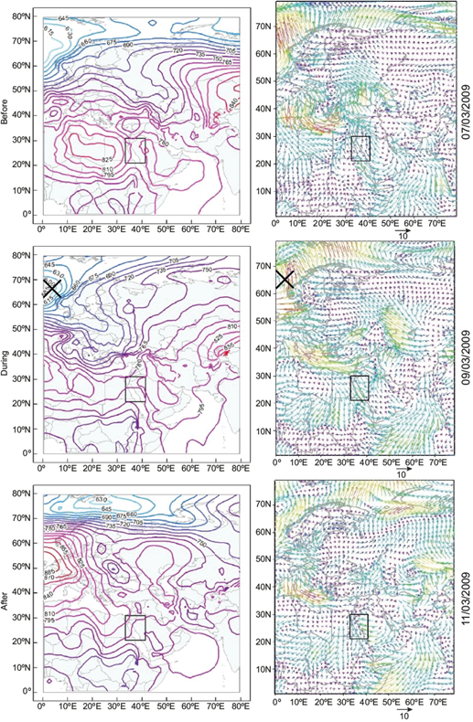
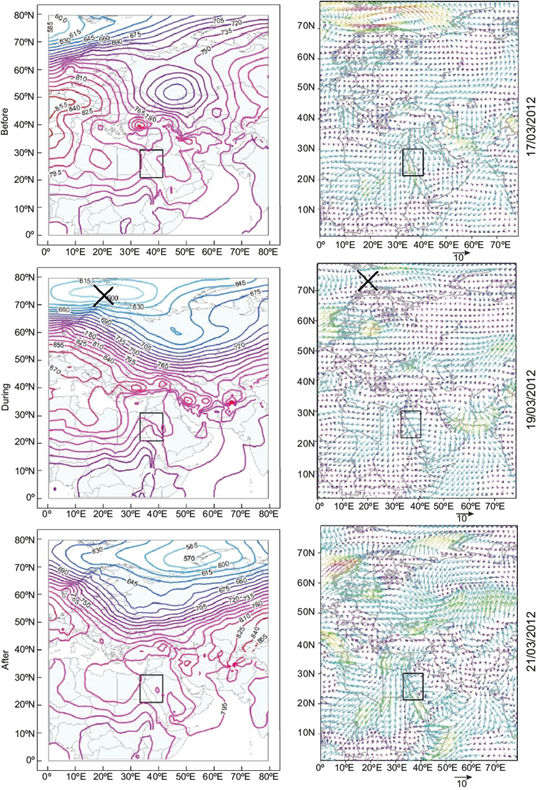
True color composite satellite images of the selected blocking and dust storm events depicting the spatial extent of the dust are presented in Figure 3. These images proceed from the Moderate Resolution Imaging Spectroradiometer (MODIS) of the National Aeronautics and Space Administration (NASA), and were downloaded from NASA’s worldview website. The black strip in images depicts the swath error (missing data) between two consecutive swath paths. The white area in MODIS images depicts clouds, whereas the light brown color represents dust storms. The spatial and temporal resolution of MODIS images is 500 m and 3-7 days. The time of image acquisition is approximately 10:30 LT.
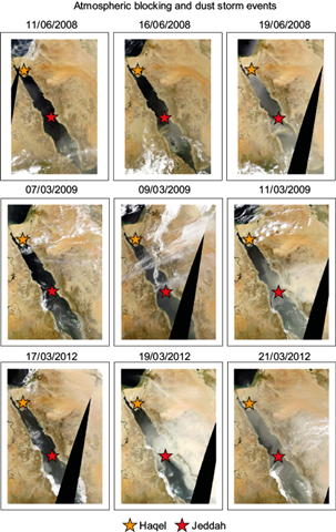
Fig. 3 MODIS satellite-based images for an atmospheric blocking event during June 2008 (top row panels), and dust events during March 2009 (middle row panels) and March 2012 (bottom row panels) (see also Fig. 1 and Table II).
Commonly used statistical measures such as mean, standard deviation and linear regression fits based on ordinary least square method, are employed to assess the relative changes in air pollutants and meteorological variables during the study period (Wilks, 2020).
3. Results and discussion
3.1 Diurnal, monthly and seasonal variations
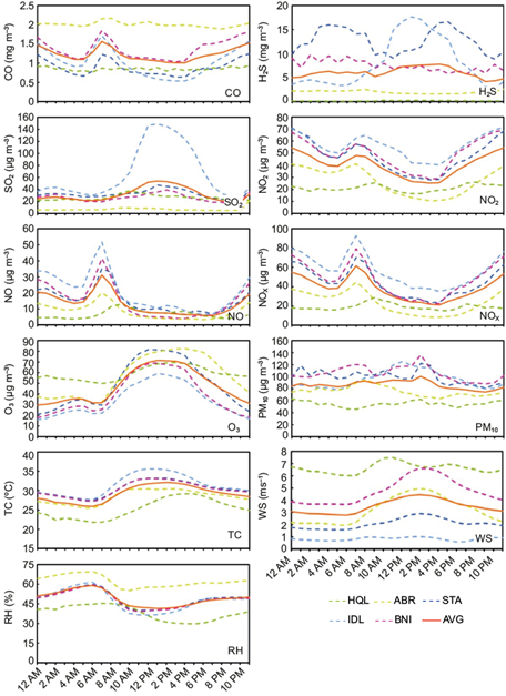
On the diurnal time scales, NO2, NO and NOX concentrations were higher during the traffic rush hours (7:00 to 9:00 LT) and in the evening. Low concentrations were observed during midday caused by high TC and an increase in photochemical production of O3 (Fig. 4 and Fig. S1 in the supplementary material). Alghamdi et al. (2014) observed a similar diurnal cycle of NO and NO2 with peak concentrations at 6:00 to 8:00 LT in spring, autumn and winter, and 24:00-2:00 LT and 5:00-6:00 LT during summer with a decreased concentration in late afternoon and then an increase in nighttime. The highest O3 concentrations were observed during the afternoon when faster winds blow due to an increase in TC. Analysis of extreme values of O3 indicated that high values are related to high WS during day time.
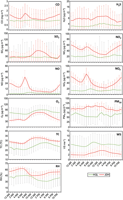
Fig. 4 Hourly variations of air pollutants and meteorological variables for Haqel (HQL) and Jeddah (JDH), including their one sigma standard deviation values, during 2008-2012. JDH shows the average of ABR, STA, BNI and IDL stations values.
Lowest O3 concentrations were recorded at 7:00 LT, i.e., during the rush hour and with increased emission of NOX. The diurnal variation of CO was similar to NOX with peak concentrations during rush hours, while SO2 exhibited a single concentration peak during during afternoon hours (12:00 to 18:00 LT). A similar SO2 behavior was noticed during winter months in Bhubaneswar, India during 2010-2012 (Mallik et al., 2019). Only IDL exhibited peak concentrations in H2S in afternoon hours. A temporal heterogeneity was observed in PM10 concentrations at all stations, however, on average, high concentrations were observed during daytime, when high TC causes an increase in WS. The diurnal trend in meteorological variables was also observed with maximum (minimum) TC observed during 8:00 to 16:00 LT (4:00 to 5:00 LT). It was found that WS increases during afternoon hours.
Monthly variations of air pollutants and meterorological variables are displayed in Figure 5. Monthly high averages of NO2, NO and NOX were observed in the warmer months (April, May, June) especially in the IDL station. Monthly fluctuations were observed for NO with high concentrations during spring and winter. The highest O3 concentrations occurred from May to August, which are the months of high TC. Alghamdi et al. (2014) found that O3 concentrations strongly follow variations in TC and observed the highest daytime average O3 concentration in August (86.43 µg m-3) and the lowest in December (46.06 µg m-3).
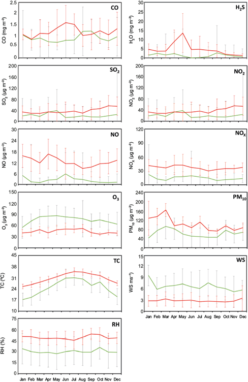
CO higher (lower) concentrations were observed in May-July (November-February). High concentrations of CO during summer can be attributed to high dispersion of CO due to dry conditions, relatively high wind speeds, and reduced wet scavenging of CO due to a low rainfall rate.
The monthly variations of SO2 and H2S exhibited spatial inhomogeneity across the stations. High concentrations of SO2 were observed for the IDL station, however, no clear pattern was observed for the remaining stations. Peak monthly concentrations for H2S were observed in April-June for the IDL and BNI stations. H2S concentrations were constant for the ABR and HQL stations. The STA station displayed a different monthly pattern due to high concentrations recorded during May-September in 2008. PM10 peak concentrations were observed during February-April, the time period of dust storm activities in the region (Shalaby et al., 2015).
The monthly variations of TC exhibited an increase (decrease) during April-October (November-February). The monthly variations of PR were opposite to those of TC, with lowest PR during June-August. RH and WS averages were relatively constant in all months, with higher RH in the ABR station, located in a coastal area. RF occurred in December-April. Dry conditions prevailed during the rest of the months (Athar, 2015).
3.2 Weekend effect
The weekend effect of air pollutants was computed for all stations using Friday as weekend and Saturday to Thursday as weekdays, following the discussion in section 2.2.2 (Fig. 6). The weekend effect for CO, NO2, NO and NOX was observed in all stations where concentrations were higher during weekdays than in weekends, except for the ABR station, which has high concentration on weekends. The difference between weekends and weekdays was highest at the IDL station.
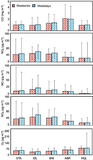
Fig. 6 Weekdays-weekends differences for CO, NO2, NO and NOx, and O3 (from top to bottom average concentrations, including their one sigma standard deviation, for each station during 2008-2012.
Low O3 concentrations on weekdays were detected for all stations except for ABR, where averages for weekdays were greater than weekends. Baidar et al. (2015)) reported similar results for California in the USA. The opposite trend was observed for the ABR station due to high vehicular emissions on weekends owing to tourism activities, as this station is located near the shore. High concentrations of O3 on weekends were recorded since this station had low NO levels, which indicates that O3 scavenging from NO was lower, resulting in higher O3 levels. The weekend effect was not observed for other air pollutants in the region.
O3 and the NOX are recognized as pollutants associated to reduced anthropogenic activities on weekends in several regions of the world, such as in California (Qin et al., 2004), Greece (Paschalidou and Kassomenos, 2004), the Iberian Peninsula (Jiménez et al., 2005), southern California (Gao et al., 2005), Japan (Sakamoto et al., 2005), Nepal (Pudasainee et al., 2006), Mexico (Stephens et al., 2008), Egypt (Khoder, 2009), and China (Wang et al., 2014).
3.3 Annual variations
The average NO2 concentration is decreasing at a rate of -1.97 µg m-3 per year (R2 = 0.47). NO and NOX concentrations are decreasing at rate of -1.73 µg m-3 per year (R2 = 0.83), and -2.42 µg m-3 per year (R2 = 0.63), respectively. All stations except IDL displayed a decreasing trend, indicating increased NOX emissions from industries. The increase rate for the IDL station is 11.08 µg m-3 per year (R2 = 0.73). The O3 average concentration for all stations is increasing at a rate of 2.99 µg m-3 per year (R2 = 0.46). In Saudi Arabia, this annual increasing rate of O3 is somewhat higher than that reported for several east Asian countries (Jung et al., 2018) and in Cyprus (Pikridas et al., 2018). The O3 concentration exhibited an inverse trend with its precursor (NOX). This behavior was also observed by Mayer (1999), who found that O3 displayed a long-term increase while a decreasing trend was found for other air pollutants.
The annual CO concentrations of all stations were found to be decreasing at a rate of -0.03 mg m-3 per year (R2 = 0.62). Similarly, a decrease in H2S and SO2 concentrations is observed. The average trend of H2S and SO2 for all stations was -514.91 µg m-3 per year (R2 = 0.87) and -6.21 µg m-3 per year (R2 = 0.89), respectively.
The PM10 average concentration for all stations was found to be increasing at a rate of 9.55 µg m-3 per year (R2 = 0.65). The increase in PM10 concentrations within the region can be attributed to dust storm events that cause substantial increase in concentrations owing to air pollutant loading (Alghamdi et al., 2015). Dust events in Saudi Arabia occur all year round with maximum intensity in spring and summer (Shalaby et al., 2015). PM10 displays high concentrations during the February-August, since 75% of dust events identified in this study were observed in those months.
3.4 Percentile based changes
The percentiles of O3 on an hourly time scale showed an increase in all stations except for BNI and HQL (Fig. 7a). An increase in O3 background values (lower percentiles) was observed in both dry and wet seasons. The behavior of stations BNI and HQL can be attributed to their suburban localization, which implies less sources of air pollutant emissions. High values of solar radiation in summer and during day time lead to higher O3 concentrations. The higher percentiles of O3 exhibited relatively large changes; similar changes were observed in its precursors’ (NO2, NO and NOX) and meteorological variables (TC and WS). High concentrations of O3 occur in response to an increase in TC and WS (Camalier et al., 2007; Shen and Mickley 2017). The 99th percentile did not exceed the EPA standard of 150 µg m-3 for the 3-year period, indicating that O3 concentrations were within the air quality standard’s limit.
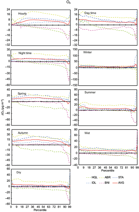
Fig. 7a Hourly daytime, nighttime and seasonal (winter, spring, summer, autumn, wet and dry) time scale percentile changes for variable O3 between the two halves of the study period (2008-2012).
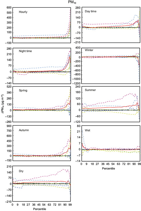
The hourly PM10 concentrations exhibited an increase in higher percentiles for all stations (Fig. 7b). Increased PM10 concentrations were observed at higher percentiles (85th and above) with a similar behavior for WS values. Minimum changes were observed in autumn and the wet season. During summer and the dry seasons, PM10 concentrations were observed increasing until the 90th percentile and then decreasing with higher percentiles. In the 1st quartile, the highest concentrations were recorded in spring and summer for most stations. PM10 concentrations exceeded the air quality standards values of during summer at the BNI station, where the median value was higher than 150 µg m-3 during the second half of the study period.
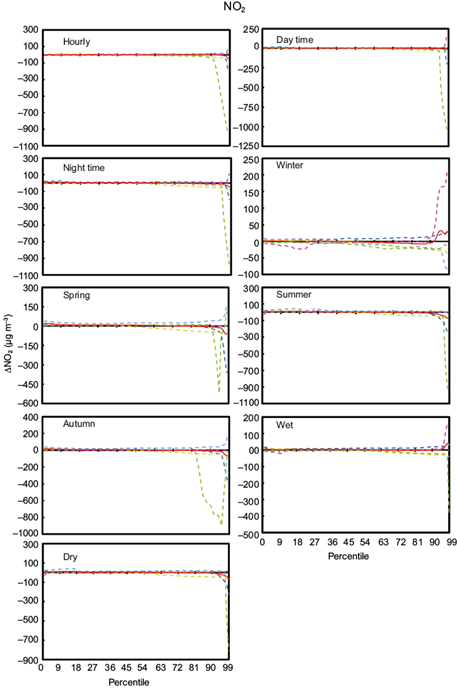
NO2, NO and NOX showed relatively small or no changes in lower percentiles and larger changes in higher percentiles (Fig. 7c). Only one station (BNI) displayed an increase above the 90th percentile for NO2 and NOX in winter. The 99th percentile did not exceed the air quality standard of 188 µg m-3 for stations STA and HQL in the first half of the study period.
The CO concentration increased in the second half of the study period for all time scales except for the wet season between the 1st to 3rd quartiles; however, a decrease in higher percentiles is observed for all time scales indicating a decrease in occurrence of high CO concentrations (not shown). The value of the 99th percentile in the studied time period was well below the EPA standard of 40 mg m-3.
SO2 and H2S concentrations decreased in the second half of the study period for the dry season, contrary to their increase during the wet season for all percentiles (not shown). The 1st, 2nd and 3rd quartiles of SO2 concentrations did not exceed the USA-EPA 24-h average standard of 365 µg m-3 . The H2S hourly average was compared to the California Ambient Air Quality Standard (due to the unavailability of a USA-EPA air quality standard for H2S), and daily concentrations were found to be higher than the standard of 45 µg m-3 for the STA station during the first half of the study period and for the ABR station in the second half. Values for the median and 3rd quartile exceeded the standard on all stations except ABR, and in the second half exceeded the standard only for ABR station.
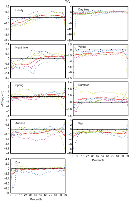
The percentile-based changes in meteorological variables provide an insight into the short-term climatology of the region. The lower percentiles for TC, PR and WS decreased in the second half of the study period, while an increase was observed for RH. Conversely, higher percentiles were found increasing (decreasing) for TC, PR and WS (RH). In the wet season, a decrease in TC and PR is observed with an increase in higher percentiles of RH indicating chances of extreme weather events. Percentile based changes on multiple time scales for TC between equal halves (during 2008-2010) are displayed in Fig. 7d.
3.5 Relation of elevated PM 10 concentration and dust storms
Several short- and long-term case studies carried out in different countries of the East Mediterranean basin found a relationship between dust storms and various indicators of air quality (Ackerman and Cox, 1989; Draxler et al., 2001; Kutiel and Furman, 2003; Zender and Kwon, 2005; Nastos, 2012; Sharma et al., 2012; Gherboudj and Ghedira, 2014). In this study , in situ atmospheric conditions and satellite-based AOD were assessed for a total of 12 events identified in a 5-year period to study the relationship between occurrence of dust storms and modulation of air pollutants in Saudi Arabia. Only eight of these events occurred during spring (February-April). Two of these cyclonic events, both of which were studied earlier, are briefly discussed next as illustrative examples, providing additional complementary information. For details of the remaining six cyclonic events, see Tazeem (2018).
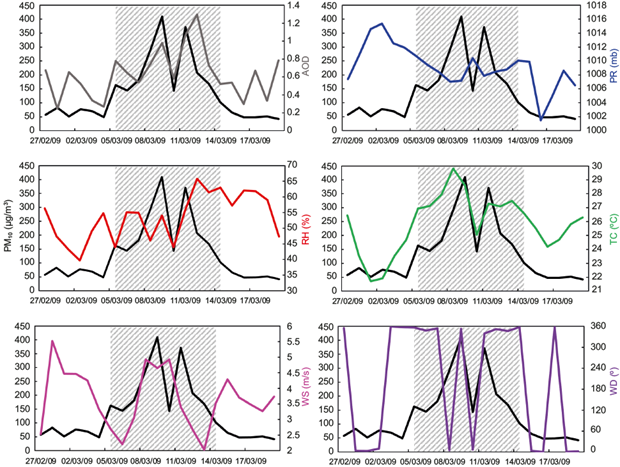
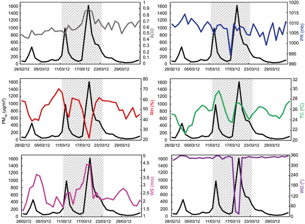
One of the studied events, identified by Alharbi et al. (2013), occurred during March 5 to 14, 2009 (Figs. S2 an S3). The storm was caused by the presence of a cold front with an upper-level jet. Dust storm events are triggered by a low PR trough produced by presence of jet stream in the region (Hermida et al., 2018). The other studied event, which occurred during March 11 to 23, 2012, was analyzed by Prakash et al. (2015), who assessed the impact of dust events on radiation fluxes and local climate characteristics (Figs. S4 and S5). A low PR system was located at 30º to 80º N that resulted in drop of PR, TC and RH and an increase in surface WS, which ranged from 3 to 8 m s-1 during the event with essentially a two-peak structure in PM10 concentration (Reizer and Juda-Rezler, 2016). Beegum et al. (2018) observed that dust emissions are strongly related to WS, hence accurate meteorological parameters are crucial for dust storm identification and air pollutants simulations. An approximate co-variation of WS and PM10 was also noted in Wuhan, China, based on in-situ observations on a daily basis during 2013-2016 (Zhang et al., 2018b). An increase in AOD was also observed with simultaneous increase in PM10 concentrations. Maghrabi and Alotaibi (2018) attributed the AOD increase during spring to the impact of dust events. Most of the events observed in the study exhibited a two-peak structure in PM10 concentrations. Similar elevated air pollutant concentrations were observed in the remaining six events.
3.6 Blocking impacts on air pollutant concentrations
Anticyclonic atmospheric blockings are events linked with persistent high PR that leads to extreme weather conditions such as heat waves, cold waves and severe air pollution episodes (Sitnov et al., 2017; Sitnov and Mokhov, 2017). Webber et al. (2017) found a strong association between blocking events over western Europe and PM10 concentrations over the UK in winter.
In the present study, a total of 26 events were identified, of which 19 occurred during the summer (May-October). Fourteen of these events displayed a significant positive deviation in geopotential height at 500 hPa (H500) from the 5-year mean during blocking periods. Likewise, seven out of the 26 were identified during winter (November-December and February). Six of them displayed significant negative deviation from the 5-year H500 mean. In this study, 14 blocking events with positive deviation from the mean were further investigated to identify significant changes in air pollutant concentrations: AOD, O3, NO2 and SO2 as well as H500 and geopotential height at 1000 hPa (H1000). It was found that 12 blocking events resulted in significant changes in one or more observed variables (Table II). The main cause of these changes in parameters was found to be associated with high PR development over the study region during the blocking period. The ensuing stagnation in air leads to a decrease in WS (which was identified via in situ observations), giving rise to accumulation of air pollutants in the region.
4. Conclusions
This study presents a detailed investigation of the spatiotemporal variations in air pollutants (CO, SO2, H2S, NO2, NO, NOX, O3 and PM10) and their relationships with meteorological variables (RF, RH, PR, TC, WS, and WD) from in-situ observations for a period of five consecutive years (2008 to 2012) using 15 min observations from ground-based data of five stations; one located in city of Haqel (HQL) and four located in city of Jeddah (STA, BNI, IDL and ABR), all in Saudi Arabia. The main conclusions deduced from the study are as follows:
Most air pollutants displayed a decreasing trend except for PM10 and O3 in the region. The IDL station, located in the industrial area of Jeddah, is the only station that displayed an increase in NO2, NO and NOX emissions, indicating excessive release of nitrogen-based oxides.
High concentrations of NO2, NO and NOX were observed during high traffic rush hours (7:00-9:00 LT), whereas the lowest O3 concentrations were found at 7:00 LT. A statistically significant correlation was found between WS and O3 concentration at hourly and diurnal time scales. PM10 also disperses in the atmosphere due to high WS. High O3 concentrations occurred in May-August due to high solar radiation and high WS in summer.
Due to low WS, there is a greater chance for air pollutants to accumulate. Accumulation of pollutants such as NO can result in reduction of O3 concentrations and vice versa. Hence, in this study a statistically significant correlation was found between WS and O3 concentrations at hourly and diurnal time scales.
A percentile-based analysis showed a decrease in all air pollutants except for O3, whose lower percentiles were found increasing during the second half of the study period, and PM10 values were found increasing in higher percentiles. An increase in O3 lower percentiles indicates an increase in background values, whereas an increase in PM10 higher percentiles indicates an increase in extreme PM10 values. The PM10 concentration exceeded the USA-EPA air quality standard, while the H2S concentration exceeded air quality standards in the first half of the study period; however, a decrease was observed in the second half.
Upper air low pressure systems located at 30º to 80º N cause the drop of PR and TC, and an increase in surface WS, resulting in extreme weather events such as dust storms. During such events, PM10 high concentrations greater than 3σ were observed in the study area, relative to non-extreme weather.
Anticyclonic blocking events resulted in significant changes in air pollutant concentrations during the blocking period due to air stagnation and a decrease in surface WS, which resulted in accumulation of air pollutants.