


 nueva página del texto (beta)
 Inglés (pdf)
 Artículo en XML
 Referencias del artículo
 Enviar artículo por email
 Citado por SciELO
  Similares en
SciELO
Similares en
SciELO 
 Permalink
1. Introduction
Urban air pollution is an important environmental problem causing serious public health effects, especially in developing countries, in the lack of proper pollution control strategies. The rising urban population, dramatic growth of vehicle fleets, rapid industrial development, and fossil fuel consumption for heating and energy production are the major sources creating air pollution (Fenger, 2009). Although sulfur dioxide and particulate matter (PM) concentrations showed a decreasing trend over the last decade in Turkey (İnandi et al., 2018), PM emissions still deteriorate air quality of Turkish cities. PM10 is the subset of the PM whose aerodynamic diameter is less than 10 mm (Kampa and Castanas, 2008). PM has several important effects on ecosystems and climate. Particles enter the aquatic and terrestrial ecosystems by dry and wet depositions and alter the structure of ecosystems through reducing growth, changing the chemical composition, and changing biogeochemical cycles (Grantz et al., 2003). Due to the scattering and absorbance characteristics of particulates, they play a role in climate change (Ramanathan and Feng, 2009). Also, visibility is reduced because of particles (Wen and Yeh, 2010) and aviation traffic is threatened (Langmann et al., 2012). However, the most important adverse effects of PM are their health effects. Exposure to PM is associated with morbidity and mortality (Anderson, 2009; Caiazzo et al., 2013) predominantly due to lung cancer and chronic obstructive pulmonary disease (COPD) (Kravchenko et al., 2014). Especially older people and children are considered as the riskiest groups that could be affected by air pollution (Chapman et al., 1997). Deposition of particles in the respiratory system is generally determined by particle size. PM10 is deposited in the upper respiratory tract, while PM2.5 reaches the alveoli and may create more severe health problems (Kampa and Castanas, 2008). Increasing PM10 concentrations result in circulatory and respiratory diseases (Cruz et al., 2015). Also, exposure to PM is related to heart rate variability (Polichetti et al., 2009). Finally, Kravchenko et al. (2014) stated that decreasing asthma deaths are related to lower PM10 levels.12q
While most cities in Turkey experience PM pollution, the situation is much more serious in some cities with extensive coal use such as Zonguldak. According to the Ministry of Environment, Urbanization, and Climate Change of Turkey, air pollution is the main environmental problem in the Zonguldak city center (MEU, 2011). The complex topographic structure of the city prevents dispersion of air pollutants and inversion events occur frequently. Ambient air quality gets worse especially in winter months, when coal is used for residential and commercial/institutional heating. This region is extremely dependent on bituminous coal for domestic heating and electricity production in thermal power plants. Four thermal power plants are operating in Çatalağzı district 12 km away from the city center. There exist several studies related to the air quality in Zonguldak (Yildirim and Bayramoglu, 2006; Tecer et al., 2008a; Akyüz and Çabuk, 2009). In addition, some studies have documented air pollution and its health effects in the region. Tecer et al. (2012) analyzed the metallic composition of aerosols in Zonguldak and pointed out that coal combustion for heating was the main source of PM. Akyüz and Çabuk (2008) focused on polyaromatic hydrocarbons in PM2.5 and PM10 samples measured at the Zonguldak Bülent Ecevit University (formerly known as Zonguldak Karaelmas University) campus. They stated that the inhabitants of the Zonguldak region have been exposed to a cancer risk especially in winter times due to high benzo(a)pyrene equivalent concentrations of particle-associated polycyclic aromatic hydrocarbons (PAHs) from coal combustion. Topan et al. (2016) reported that lack of environmental precautions and comprehensive pollution control strategies is the main reason for air pollution in Zonguldak, and high cancer incidence rates including childhood cancer cases are mostly seen in the city center. Moreover, wintertime air pollutants are related to hospital admissions, consultations, and hospitalizations (Ségala et al., 2008). Tecer et al. (2008b) found a significant positive correlation between PM concentrations and hospital admissions for respiratory diseases (asthma, allergic rhinitis, upper and lower respiratory diseases) in Zonguldak. Another study emphasized the existence of a significant association between occurrence of respiratory symptoms and diseases (ORSD) and ambient levels of PM, SO2, and pollen concentrations in Zonguldak (Tecer et al., 2009). Similar results have been reported by Tağıl and Menteşe (2012), who observed a statistically significant positive correlation between concentrations of air pollutants (SO2 and PM10) and hospital admissions due to asthma, bronchitis, and COPD. Örnek et al. (2015) mentioned that high levels of PM10 due to coal-burning may have contributed to higher COPD prevalence observed in Zonguldak. Tomac et al. (2005) discovered a strong positive correlation between childhood asthma and air pollution levels, while Türk et al. (2020) stated that air pollution is the possible risk factor for multiple sclerosis (MS) disease in Zonguldak. Finally, Celik et al. (2014) investigated the patient mortality factors at the intensive care units of Zonguldak between 2006 and 2011, concluding that the highest mortality rates were due to kidney diseases, cardiovascular and respiratory system diseases. It should be noted that cardiovascular and respiratory system diseases are attributable to air pollution. In Turkey, during the Covid-19 pandemic, Zonguldak was the only city where travel restrictions were implemented besides 30 highly-populated metropolitan cities, concerning the high frequency of air-pollution-related health risks in the city. Goren et al. (2021) stated that coal mining, thermal power plants, and having a higher rate of respiratory disease in Zonguldak are the reasons for establishing travel restrictions in this area. Similarly, Dursun et al. (2021) emphasized high levels of air pollution in the province of Zonguldak.
It is obvious from the cited literature that SO2, total suspended particulate (TSP), PAHs, PM10, and their health effects are studied in the ambient atmosphere of Zonguldak. However, previous studies have not dealt with the spatial distribution of air pollutants. The present study aimed to fill this gap. The spatial distribution of pollutants can be revealed by means of air quality monitoring or air quality modeling. To obtain a high-resolution map, there should be enough air quality monitoring stations (AQMS). Also, active, or passive sampling of ambient air followed by laboratory analysis of the pollutants in a certain number of sampling points can be used for monitoring and mapping purposes, but they are costly. For these reasons, air quality modeling is chosen as the best alternative to establish spatial distribution maps. In this study, we focused on the pre-natural gas era in domestic heating to reveal the worst-case scenario for air quality in Zonguldak. The emission inventory is compiled for the year 2011. Air quality modeling is performed for the period between 2007 and 2011. For these years, there was only one air AQMS, recording only PM10 and SO2 in the area.
This study presents the spatial distributions of PM10 concentrations determined by air quality modeling including all types of sources in the Zonguldak region for the first time. Application of AERMOD and CALPUFF are common for air quality modeling studies in Turkey (Elbir, 2003; Tayanç and Berçin, 2007; Demirarslan et al., 2017; Tuygun et al., 2017). AERMOD is a regulatory model of the United States Environmental Protection Agency (US-EPA). The Turkish Ministry of Urbanization, Environment, and Climate Change enforces the use of this model in environmental impact assessment studies. However, literature states that complex models like CALPUFF perform better than Gaussian plume models like AERMOD on complex terrains near shorelines. Abdul-Wahab et al. (2011) reported that for power plants located between mountains and seashore, CALPUFF is more suitable than AERMOD to estimate pollutant concentrations. Also, Atabi et al. (2016) found that CALPUFF gives better results on complex topographical conditions for the modeling of emissions from gas refineries located near the seashore. CALPUFF algorithms include overwater dispersion and coastal interactions effects like coastal fumigation and thermal internal boundary layer (Abdul-Wahab et al., 2011). Therefore, these two models are selected and used in this study. Another aim of this study is to compare the outputs of AERMOD and CALPUFF in an elevated terrain near the shoreline.
2. Material and methods
2.1 Study area
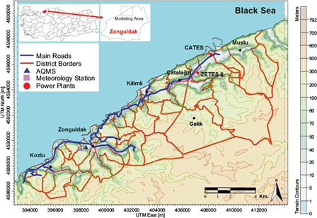
The Zonguldak province is located on the west coast of the Black Sea region in Turkey. The province is famous for coal mines and is called the land of “black diamond”. The study area, the Zonguldak metropolitan region, encompasses three counties (Zonguldak, Kozlu, and Kilimli) and three towns (Çatalağzı, Muslu, and Gelik). Çatalağzı is especially important because the coal-based thermal power plants are located there. Figure 1 shows the modeling domain, a 21 × 16 km area covering a total of 336 km2. The region is surrounded by the Black Sea to the north and by hilly terrains to the south, east, and west. Meteorological parameters play an important role in the distribution of air pollutants in the area. Topographical and meteorological conditions prevent dispersion of air pollutants; therefore, inversion events occur frequently. The meteorological station in the modeling area is located at 41.4492 N and 31.7779 E. The Black Sea climate predominates, with an annual average temperature of 13.6 ºC. July and August are the warmest months, while January and February are the coolest. The annual average rainfall is 1217.8 mm. The yearly mean wind velocity is 2.3 m s-1 and the predominant wind directions are ESE, SE, and SSE. The annual average pressure is 1000.1 hPa and the average relative humidity is 71.2% (Tecer et al., 2012; TSMS, 2019). There was only one air quality monitoring station during the modeling period (2007-2011) and the station continuously monitored ambient concentrations of sulfur dioxide (SO2) and PM (PM10). The location of the Zonguldak AQMS is also shown in Figure 1 (41.4513 N and 31.7833 E). According to the Address Based Population System, 183 651 inhabitants lived in this region in 2011.
2.2 Emission inventory
An emission inventory can be defined as a compilation of the amount of all air pollutant entering the atmosphere from all sources in a geographical area for a certain time (Elbir and Muezzinoglu, 2004). The emission inventory of this study was prepared for PM10 emissions of domestic heating, transportation, and industrial activities. Emissions of illegal fuel usage for heating were not included due to insufficient data. In this study, the PM10 emission inventory was compiled for 2011. Since official emission factors for Turkey are quite limited, they were selected from two widely known databases published by the US-EPA and the European Environmental Agency (European Environmental Agency). PM10 emissions for point and area sources were calculated by using Eq. (1).
where E is the amount of PM10 emissions (t year-1), Fueli is the activity data (total fuel consumption per year) for each fuel type, EF i is the emission factor for each fuel type and ER is the emission reduction in percentage, providing there is an air pollution control equipment. Eq. (2) was used for line sources (motor vehicle emissions).
where E is the amount of PM10 emissions (t year-1), Veh i is the number of vehicles per type, D i is the distance traveled in a year for a specific type of vehicle, and EF i,km is the emission factor per vehicle type (i) per km (Çetin et al., 2007).
2.2.1 Line sources
Motor vehicle emissions were classified as line sources in the study. The number of vehicles for each vehicle type was counted in 11 main roads within the modeling domain, since these motorways encompass most of the traffic in the modeling domain. Emission factors for each vehicle type (Table I) were taken from another study (Çetin et al., 2007) based on the Tier 2 method of the European Monitoring and Evaluation Program (EMEP)/EEA Air Pollutant Emission Inventory Guidebook.
Table I PM10 emission factors for each vehicle source*.
| Vehicle type | PM10 Emission factor (g km-1) |
| Gasoline passenger cars | 0.0011 |
| Diesel passenger cars | 0.21 |
| Minibuses | 0.21 |
| Light commercial vehicles < 3.5 t | 0.21 |
| Heavy-duty trucks < 32 t | 0.56 |
| Heavy-duty trucks > 32 t | 0.72 |
| Buses | 0.52 |
*Vehicle speed is 50 km h-1.
2.2.2 Area sources
Area sources in the modeling domain were assessed in two classes: domestic heating and ship activities in the Zonguldak harbor. The primary fuel for domestic heating was bituminous coal during the modeling period and some institutions were using fuel-oil 6. Therefore, PM10 emissions of a total of 93568 homes, 41 governmental institutions, 39 private workplaces, and 76 primary and secondary schools were included in the inventory. According to the results of the questionnaire performed by Zeydan (2008), the average coal usage values in Zonguldak for domestic heating were determined as 3.83 t year-1. Some of the private and governmental institutions (schools, governorship, municipality, police headquarters, gendarmerie, etc.) were using fuel-oil 6 for heating during the study. Their fuel consumption values were directly obtained from the Zonguldak Provincial Environmental Directorate. PM10 emissions of ships in the harbor were taken from the study of Kocabaş et al. (2012) as 8.40 t year-1. Emissions from illegal coal consumption and quarries could not be included in the inventory because of insufficient data. Emission factors for area sources (heating activities) were obtained from the AP-42: Compilation of air emissions factors published by US-EPA (1997). PM10 emission factors for sources that burn coal and fuel-oil 6 are presented in Table II after unit conversion.
2.2.3 Point sources
Zonguldak is one of the leading provinces in terms of industrialization in the Black Sea region. There are two organized industrial zones in Zonguldak but none of them is in the modeling region. The only industrial emission sources in the study area are thermal power plants in the Çatalağzı energy basin. Currently there are four thermal power plants settled in the area, with a total capacity of 3104 MW: Çatalağzı (CATES) (2 × 157 MW), Zonguldak Eren I (ZETES I) (160 MW), Zonguldak Eren II (ZETES II) (2 × 615 MW) and Zonguldak Eren III (ZETES III) (2 × 700 MW). During the modeling period, only CATES and ZETES II were operating. ZETES I was out of service, so it was not included in the emission inventory and modeling. ZETES III has been operating only since 2016. Thus, this power plant was neither included in the 2011 inventory calculation nor in the modeling study. Also, emissions from coal transport and storage facilities, and ash dams of thermal power plants could not be added to the inventory due to lack of data. Fuel consumption data and stack information were obtained from environmental impact assessment reports of these power plants. CATES yearly consumes 1600000 t of coal as a primary fuel and 7200 t of fuel-oil 6 (with a sulfur content of 2.8%) as a secondary fuel. Low-quality coal with a poor heating capacity of 3300 kcal kg-1 and ash content of 45% was used in CATES. The particulate removal efficiency of the air pollution control equipment of the plant is given as 98% (Çınar Engineering, 2009). On the other hand, ZETES II is the first supercritical pulverized coal power plant in Turkey. At peak load, it consumes yearly 3440000 t of coal as primary fuel and 45000 t of fuel-oil 4 as secondary fuel. Hence, it was assumed that ZETES II works at its peak capacity, and inventory calculations were performed consequently. The lower heating capacity of coal burnt at ZETES II is 6500 kcal kg-1 with an ash content of 10%. The efficiency of the electrostatic filter is given as 99.6% for particulates (Çınar Engineering, 2009). Emission factors for point sources were obtained from US-EPA’s AP-42: Compilation of air emissions factors (US-EPA, 1997) and listed in Table III . The stack characteristics of these power plants are given in Table IV.
Table III PM10 emission factors for point sources.
| CATES | ZETES II | |||
| Coal | Fuel-Oil 6 | Coal | Fuel-Oil 4 | |
| US-EPA EF | 2.3A lb ton-1 | 9.19S + 3.22 lb 1000gal-1 | 2.3A lb ton-1 | 7 lb 1000 gal-1 |
| Derived EF | 47 kg ton-1 | 3.52 kg ton-1 | 10.44 kg ton-1 | 3.18 kg ton-1 |
EF: emission factors; S: sulfur content; A: ash content.
The density of Fuel-Oil 6 is 0.9861 kg l-1, the density of Fuel-Oil 4 is 0.95 kg l-1.
Table IV Stack characteristics of power plants.
| Power plant | CATES | ZETES II |
| x coordinate (m) | 408220.1 | 407180.9 |
| y coordinate (m) | 4596773.1 | 4595311.0 |
| Base elevation (m) | 6 | 10 |
| Stack elevation (m) | 126 | 190 |
| Exit gas temperature (ºC) | 158 | 80 |
| Stack inside diameter (m) | 6.2 | 6.5 |
| Exit gas velocity (m s-1) | 5.29 | 14.9 |
| Exit gas flow rate (m3 s-1) | 159.7 | 494.4 |
2.3 Air quality modeling
Air quality modeling is the mathematical simulation of the destination of air pollutants after release from source to receptor points including their movements (transport and dispersion), reactions, and removal (dry and wet deposition) processes (Holmes and Morawska, 2006). The Gaussian dispersion model explains the dispersion of plume concentration in the vertical and horizontal axis perpendicular to the wind direction (Fraile et al., 2006). On the other hand, puff models are used to model dispersion and movement of discrete emissions (series of puffs over time) from the stack. The Gaussian puff model successfully calculates pollutants concentrations in case of low wind speeds while the Gaussian dispersion model generally fails (Holmes and Morawska 2006; Gulia et al. 2015). Dimensions of the puff are determined with dispersion parameters, which are functions of the puff’s travel duration (Korsakissok and Mallet, 2009; Abdul-Wahab et al., 2011).
The AMS/EPA Regulatory Model (AERMOD) was developed by the American Meteorological Society (AMS) and the United States Environmental Protection Agency (US-EPA). AERMOD is one of the most widely used regulatory models. It is a near-field steady-state Gaussian plume model and can model point, area, and volume sources in flat and complex terrain (Holmes and Morawska, 2006; Yassin and al-Awadhi, 2011). Line sources can be added to AERMOD as a series of area sources. This model can calculate pollutant concentrations up to 50 km from the source. The AERMOD model formulation was well defined by Cimorelli et al. (2005) and Jeong (2011). To calculate pollutant concentrations, the Gaussian probability distribution function is used both in the vertical and horizontal axes in the stable boundary layer, and the horizontal axis in the convective boundary layer. However, vertical distribution in the convective boundary layer depends on the bi-Gaussian probability density function (Vijay Bhaskar et al., 2008; Yassin and al-Awadhi, 2011). AERMOD uses two preprocessors: the meteorological preprocessor AERMET and the terrain preprocessor AERMAP (Jeong, 2011; Kakosimos et al., 2011). Hourly meteorological data required by AERMET are cloud cover, temperature, relative humidity, pressure, wind direction, wind speed ceiling height, precipitation, and horizontal radiation. AERMET also needs some surface parameters like albedo, Bowen ratio, and surface roughness. Then, it uses the planetary boundary layer theory and calculates planetary boundary layer parameters like Monin-Obukhov length, friction velocity, sensible heat flux, and convective scaling velocity. With the help of these parameters, convective velocity scale and mixing height can be estimated (Cimorelli et al., 2005; Kakosimos et al., 2011). The terrain preprocessor AERMAP is used for calculating terrain heights at receptor points (Heckel and Lemasters, 2011; Kakosimos et al., 2011).
Another air quality model used in this study is The CALifornia PUFF (CALPUFF) model developed by Sigma Research Corporation. CALPUFF is a non-steady-state Lagrangian Gaussian puff model (Indumati et al., 2009). Gaseous and particulate pollutants can be modeled by CALPUFF using space and time-varying meteorological conditions. CALPUFF can model point, area, and volume sources. Like AERMOD, line sources can be added as a series of area sources in this model. The CALPUFF formulation calculates partial penetration, buoyant and momentum plume rise, stack and building effects, dry and wet deposition (Holmes and Morawska, 2006; Abdul-Wahab et al., 2011). CALPUFF has three components: CALMET preprocessor, CALPUFF, and CALPOST postprocessor. CALMET calculates hourly meteorological data and wind fields, while CALPOST is used to calculate averaging and reporting concentrations depending on CALPUFF results (Barna and Gimson, 2002; Oshan et al., 2006). Details of the CALPUFF model formulation can be found in Jeong (2011) and Scire et al. (2011).
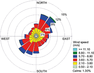
In this study, AERMOD View and CALPUFF View software, developed by WebLakes, was used for modeling. PM10 emissions of two thermal power plants, 11 main roads, 44 districts, and the harbor were entered as source inputs in both models. Area sources of residential heating were effective only in the heating season (from October 15 to May 15). Receptors were defined as a rectangular grid with 250 m between adjacent receptors. In total, 3576 receptor points were placed in the modeling domain. All sources and receptors were placed by using Universal Transverse Mercator (UTM) projection (Zone 36 North) on WGS-84 Datum. The same configuration of sources and receptors was applied for both models. Five years (2007-2011) of AERMET and CALMET ready meteorological data (hourly surface and upper air) were obtained from WebLakes. The reason for using 5 years of meteorological data was to increase the accuracy of forecasting. The wind rose plot of the given years is provided in Figure 2. Surface parameters of the modeling area, required by the AERMET preprocessor, are shown in Table V. Since the modeling region consisted of three different land-use types (sea, forest, and urban area), weighted averages of surface parameters were determined and used in the AERMET preprocessor. Although AERMOD View provides digital terrain data from United States Geological Survey (USGS) web server, global digital elevation model (GDEM) data obtained from the Advanced Spaceborne Thermal Emission and Reflection Radiometer (ASTER) sensor, onboard the Terra satellite was used due to GDEM’s better resolution (30 × 30 m). ASTER GDEM files can be freely obtained from the NASA Earthdata website (Earthdata, 2020). In the CALPUFF model, a geophysical preprocessor is necessary to obtain the geophysical data file (geo.dat) required by CALMET. ASTER GDEM’s digital terrain data were used for topography. These files were converted into 7.5 min DEM format to run them with a geophysical processor. A 1 × 1 km grid resolution was applied t meteorological grids, producing 21 cells along the x-axis and 16 cells along y-axis. Ten vertical cells were applied, and default settings were used for cell face heights (0, 20, 40, 80, 160, 320, 640, 1200, 2000, and 3000 m). The Diagnostic Wind Module option was selected from the Wind Fields options. The diagnostic model allows certain features of the flow field such as sea breeze circulation with return flow aloft (Scire et al. 2011). After that, the CALMET preprocessor and CALPUFF model were run. The final step in the CALPUFF modeling system was the CALPOST postprocessor which is used to calculate pollution concentrations for selected averaging times. Both AERMOD and CALPUFF models were run for 1 and 24 h, and annual averaging times.
2.4 Determination of model performance
Fractional bias (FB) (Eq. 3), index of agreement (IA) (Eq. 4), geometric mean bias (MG) (Eq. 5), and geometric mean-variance (VG) (Eq. 6) are widely used statistical parameters for the determination of model performance in air quality modeling studies (Chang and Hanna, 2004; Donnelly et al., 2009; Paschalidou and Kassomenos, 2009; Behera et al., 2011; Amoatey et al., 2018). A perfect model has IA, MG and VG = 1, and FB = 0 (Jeong, 2011). The FB value falls in the interval of ENT#091;-2, 2ENT#093;. Negative FB represents the over-predicting model whereas positive FB means the under-predicting model (Behera et al., 2011). Hanna and Chang (2012) stated that an acceptable model should have -0.3 ≤ FB ≤ 0.3 for rural areas and -0.67 ≤ FB ≤ 0.67 for urban areas. IA can be defined as the normalized measure of model prediction errors and varies between 0 and 1. Higher IA values (close to 1) represent an acceptable performance (Moriasi et al., 2007). IA ≥ 0.5 is considered a good performance (Amoatey et al., 2018). Acceptance criteria for geometric mean and geometric variance are 0.7 < MG < 1.3 and VG < 1.6, respectively (Chang and Hanna, 2004; Donnelly et al., 2009).
where O is observed concentrations, P are predicted concentrations, and O̅ and P̅ are the means of observed and predicted concentrations. Finally, n is the amount of data. To determine the model performance, daily averages of PM10 concentrations measured at Zonguldak AQMS between 2008 and 2011 were used in this study. For that period, this station’s records were published as raw and un-validated measurements. Therefore, outliers were removed from the dataset by examining the box plots. A discrete receptor was placed to obtain concentration values for the AQMS. After that, the only missing information was the background PM10 concentration value (the pollution due to natural sources and far anthropogenic sources). For this, the histogram of PM10 concentrations was drawn, where the peak point of the histogram represents the background concentration. Finally, model predictions plus background concentration were validated against measured concentrations.
3. Results and discussion
3.1 Emission inventory results
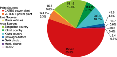
Before employing air quality modeling it is necessary to represent the emission inventory results. The results of the PM10 emission inventory are given in Figure 3, according to which a total of 2710.2 t of PM10 emissions were released into the Zonguldak atmosphere annually, and CATES thermal power plant was found as the main source of particulate pollution in the study area. Total emissions of the power plants (CATES and ZETES II) were calculated as 1648.7 t year-1 (60.8% of total emission). On the other hand, domestic heating (together with harbor emissions) accounted for 38.6% of the total emission. Domestic heating emissions of PM10 for Zonguldak, Kilimli, Kozlu, Çatalağzı, Muslu, and Gelik were determined as 531.5, 151.9, 283.4, 43.8, 10.0, and 16.7 t year-1, respectively. Motor vehicle emissions were only a small portion (0.6%) of the total emissions. There is only one previous study in the literature (Tecer et al., 2008a) that provides a PM10 emission inventory for Zonguldak, in which the total PM10 emission amount was reported as 17170 t year-1. According to this inventory, 11000 t of PM10 resulted from the emission of the Erdemir steel factory, but this source was not included in our study since it is approximately 37 km outside the modeling domain. Tecer et al. (2008a) included all registered cars (with total emissions of 315 t year-1) in their inventory. On the other hand, they only included 11 main roads regarding traffic emissions, together with the emissions of 55000 homes and workplaces (which were calculated as 355 t year-1). In our inventory, 93568 homes and 156 public and private workplaces were included. Moreover, they did not address the details of the inventory (such as emission factors), therefore it is not possible to make an exact comparison between the two inventories.
3.2 Air quality modeling results
Having represented the emission inventory results, this section provides the results of air quality modeling. Maximum concentrations are obtained from AERMOD and CALPUFF models for 1 and 24 h, and 1-year averaging times. Table VI presents the maximum concentrations and their locations. As seen from this table, the CALPUFF model outputs are much higher than AERMOD. The maximum PM10 concentrations predicted by CALPUFF are 743.2, 236.5, and 37.3 µg m-3 for 1 h, 24 h, and 1-year averaging times, respectively. On the hand, AERMOD gives 364.2, 105.1, and 17.2 µg m-3 values for the same averaging times. In literature, several studies compotherared AERMOD and CALPUFF models with respect to model performance. Tartakovsky et al. (2016) performed air quality modeling in complex terrain and suggested using AERMOD instead of CALPUFF for regulatory purposes to better protect the population. However, their modeling area was located to the west of Jerusalem and away from the shoreline. Amoatey et al. (2018) conducted a health risk assessment study in a coastal area with flat terrain and reported that AERMOD predictions were better than CALPUFF. On the other hand, according to the results of this study, CALPUFF predictions were higher than those of AERMOD. The higher concentrations of the CALPUFF model may result from recirculation of pollutants. Sea breezes (also called day breezes) and thermal internal boundary layers are the sources of the recirculation process; they occur because of the thermal contrast between dry land and sea (Efimov and Barabanov 2009; Shang et al. 2019). Levy et al. (2009) mentioned that coastal recirculation adversely affects air pollution concentrations. Indumati et al. (2009) stated that sea breeze could increase ground-level concentrations near the coastal regions. Although CALPUFF does not include a specific sea breeze module, a diagnostic wind module option was used in this study. Therefore, the effects of sea breezes can be determined by the CALPUFF modeling system. Moreover, the CALPUFF model has a specific algorithm to handle overwater dispersion and coastal interactions (coastal fumigation and thermal internal boundary layer), so that the impacts of coastal fumigation can be revealed easily. The complex topography and coastal fumigations create complex meteorological conditions which can be handled more easily by the CALPUFF model (Abdul-Wahab et al., 2011). Bluett et al. (2004)) suggested that using advanced models like CALPUFF for coastal areas can provide a better simulation of the fumigation process. As a result, it can be said that AERMOD underpredicts concentrations as compared to CALPUFF on shoreland with complex topography, while CALPUFF gives better results on complex topographical conditions for modeling emissions from gas refineries located near the shoreline (Atabi et al. 2016). Therefore, advanced models like CALPUFF should be preferred over AERMOD for environmental impact studies of emission sources located in seashore and hilly regions.
Table VI The model predicted maximum PM10 concentrations (µg m-3) and their locations.
| Averaging time | Model | Maximum concentration (µg m-3) | x coordinate (m) | y coordinate (m) | District |
| 1 hour | AERMOD | 364.2 | 393500 | 4587000 | Fatih (Kozlu) |
| CALPUFF | 743.2 | 405500 | 4591750 | Subatan (Kilimli) | |
| 24 hours | AERMOD | 105.1 | 398500 | 4590000 | Harbor |
| CALPUFF | 236.5 | 397750 | 4589000 | Terakki (Zonguldak) | |
| 1 year | AERMOD | 17.2 | 398500 | 4590250 | Harbor |
| CALPUFF | 37.3 | 397500 | 4589000 | Terakki (Zonguldak) |
The initial objective of this study was to determine polluted zones by air quality modeling. PM10 distribution maps are displayed in Figure 4a-d for 1 and 24 h averaging times for both models. It is apparent from Figure 4 that CALPUFF predicted higher concentrations as compared to AERMOD, which reports the maximum concentration (364.2 µg m-3) at Fatih district of Kozlu county for 1 h averaging time, while CALPUFF predicted the maximum concentration as 743.2 µg m-3 at Subatan district of Kilimli county, west of Gelik, for the same averaging time. As seen from Figure 4a, the most polluted region is Kozlu, and polluted areas are close to the seashore in AERMOD. However, CALPUFF gives results (Fig. 4b) for different hotspot areas where PM10 concentrations are higher than 400 µg m-3. Kallos et al. (2000) investigated sea breezes on the Black Sea and emphasized that strong sea breezes are observed over the Turkish coast during the day. They also reported that urban plumes of Istanbul disperse to the SW direction. The location of Zonguldak is close to Istanbul and similar wind patterns can be expected. The thermal power plant emissions in the modeling domain may disperse to the central region, explaining the higher concentrations and hotspots of particulate matter emissions in CALPUFF results. In Figure 4c, 24-h averaging time concentrations of AERMOD show similar patterns as in the 1-h averaging time concentrations (Fig. 4a). The maximum concentration (105.1 µg m-3) occurs at Zonguldak harbor and the surrounding region (city center). For the same averaging time, the CALPUFF model’s peak concentration is seen at the Terakki district of Zonguldak county (236.5 µg m-3) (Fig. 4d). The daily PM10 limit established by the World Health Organization (WHO) and the European Union (EU) is 50 µg m-3 (Zeydan and Pekkaya, 2021). As seen from Figure 4c, d, the highest concentrations are above this threshold value.
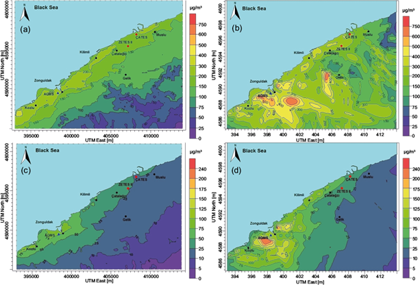
Fig. 4 PM10 pollution distribution maps. (a) AERMOD model output for 1-hour averaging time. (b) CALPUFF model output for 1-hour averaging time. (c) AERMOD model output for 24-hours averaging time. (d) CALPUFF model output for 24-hours averaging time.
The air quality modeling results of this study are especially important in terms of the Çatalağzı region. The CATES thermal power plant was installed in 1948 and renewed in 1991. However, due to its old technology, CATES could not meet air quality regulations and it was on the focus of environmentalists. In the last two decades, this region was considered as an energy basin by the Ministry of Energy and Natural Resources. ZETES I and II were installed in 2010 in the Çatalağzı region. It is obvious from the modeling results that PM10 emissions of thermal power plants together with domestic heating emissions create unhealthy ambient air conditions for the people in Zonguldak. According to the recent report of the Health and Environment Alliance (HEAL), emissions of CATES and ZETES II thermal power plants may be related to 1100 and 1412 premature deaths, respectively (HEAL, 2021), suggesting the need of taking urgent precautions for public health. It should be also noted that ZETES I was under maintenance and was not included in air quality modeling for the year 2011. However, in 2016, another thermal power plant called ZETES III (700 × 2 MW) was installed close to the other plants and the total capacities of the ZETES power plants reached 2790 MW, making them the largest in Turkey with respect to capacity. Currently ZETES (I, II, and III) and CATES produce 7% of the total electricity of Turkey (Cardoso and Turhan, 2018). Perhaps the most important finding of this study is that the Çatalağzı region should be considered as polluted in terms of particulate pollution and no more thermal power plants should be installed in this region.
As stated earlier, this work is the first detailed air quality modeling study in the Zonguldak province that shows the spatial distribution of PM10 concentrations. So, it is not possible to compare the results of this paper to previous studies in the same modeling area. Therefore, we examined the maximum PM10 concentrations of air quality modeling studies of other cities in Turkey. Elbir et al. (2010) used the CALPUFF model and reported the maximum annual PM10 concentration as 90 µg m-3 for Istanbul. In another study, the CALPUFF model predicted the maximum annual PM10 concentration as 276 µg m-3 in Izmir (Elbir, 2004). Both cities are highly populated and heavily industrialized as compared to Zonguldak. Considering that CALPUFF estimated the maximum annual PM10 concentration as 37.3 µg m-3, it could be said that the annual maximum PM10 levels in Zonguldak province are not as high as that of metropolitan cities like Istanbul and Izmir.
3.3 Model performance evaluation
The last but not least issue regarding air quality modeling studies is model performance evaluation. Model-predicted plus background concentrations are validated against daily measured PM10 concentrations at Zonguldak AQMS between 2008 and 2011. The total dataset contains 1186 observations after the elimination of outliers. The background concentration was not given as an input for both models since it was aimed to predict PM10 pollution distribution from known sources in the modeling area; nevertheless, as stated earlier, some PM10 sources (illegal coal use, quarries, coal transport, storage facilities, and ash dams of thermal power plants) could not be included in the inventory study. Moreover, re-suspension of particulates from coal ash refuses by the effect of wind may have contributed to PM10 concentrations. Also, some portions of particulates may be transported to the modeling domain via long-range transport. Therefore, background concentration should be included in the model performance evaluation. Unfortunately, there was no background AQMS in the modeling area. So, background concentration was obtained by drawing a histogram of PM10 concentrations. The peak point of the histogram corresponds to background concentration. As seen from Figure 5, background concentration is determined as 49 µg m-3.
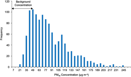
Table VII compares the model evaluation parameters for AERMOD and CALPUFF. FB values are found to be 0.30 for AERMOD and 0.28 for CALPUFF, both positive, which means that the two models underpredicted PM10 concentrations. Lee et al. (2014) found FB values ranging from 0.043 to 0.821 for PM10. Barna and Gimson (2002) reported a fractional bias ranging between -0.17 and 0.30 for PM10 for their dispersion modeling in Christchurch, New Zealand. Gibson et al. (2013) found annual, monthly, and hourly FB values for PM2.5 as 0.96, 0.88, and 0.89 for Halifax and 0.96, 0.95, and 0.90 for Pictou, respectively. Otero-Pregigueiro et al. (2018) found FB values of 0.44 in their PM10 modeling study near an industrial plant. The FB values in this study are quite reasonable compared to the literature, falling into the acceptable range of Hanna and Chang (2012) definition for urban areas (-0.67 ≤ FB ≤ 0.67). In our study, IA values were found to be 0.50 for AERMOD and 0.51 for CALPUFF, passing a good performance criterion (IA ≥ 0.5) (Amoatey et al., 2018). Elbir et al. (2010) reported lower IA values (between 0.33 and 0.50) for an air quality modeling study for PM10 in Istanbul. On the other hand, similar IA findings (in the range of 0.37-0.59) were reported by Elbir (2004) for particulate pollution in Izmir. Lee et al. (2014) reported IA values for PM10 between 0.50 and 0.85 in Ulsan, Korea. Therefore, it can be concluded that IA values in this study are consistent with the literature.
Table VII Acceptance criteria and model evaluation parameters for AERMOD and CALPUFF models.
| Model | FB | IA | MG | VG |
| Acceptance criteria | -0.67 ≤ FB ≤ 0.67 (urban) | IA ≥ 0.5 | 0.7 < MG < 1.3 | VG < 1.6 |
| AERMOD | 0.30 | 0.50 | 1.21 | 1.24 |
| CALPUFF | 0.28 | 0.51 | 1.20 | 1.24 |
FB: fractional bias; IA: index of agreement; MG: geometric mean bias; VG: geometric mean-variance.
In this study, geometric mean bias (MG) values are determined as 1.21 for AERMOD and 1.20 for CALPUFF. Song et al. (2006) reported MG values in the range of 1.01-1.83 for PM10 modeling in Beijing. MG findings in another PM10 modeling in the greater Thessaloniki area, Greece was stated as 1.17 (Kakosimos et al., 2011). MG values in this work satisfy the model acceptance rule (0.7 < MG < 1.3) and are in accordance with other studies. The last statistical parameter of performance evaluation in this study is geometric mean-variance (VG), whose values for both models were calculated as 1.24, also below the limit value (VG < 1.6). Kakosimos et al. (2011) reported VG values of 1.07 for PM10 modeling in the greater Thessaloniki area. VG values for SO2 and NO2 modeling in Tema metropolis, Ghana were found as 1.01 and 2.61 for CALPUFF, and 2.04 and 1.04 for AERMOD models (Amoatey et al., 2018). Thus, FB, IA, MG, and VG values in this study are in line with the literature and all parameters fall in acceptable ranges. Therefore, it can be concluded that both models are satisfactory, but the performance of CALPUFF is slightly better than that of AERMOD due to lower FB, MG, and VG values, and higher IA value.
4. Conclusion
Decision-makers can use air quality modeling as a useful tool for managing local air quality, selecting a proper site for air quality monitoring stations or new settlements, and preparing clean air plans for the cities. This study is the first detailed air quality modeling study performed in Zonguldak province that shows PM10 concentration distributions. A high-resolution emission inventory was prepared for this purpose. PM emissions for two coal-burning thermal power plants, 93568 homes and 156 public and private workplaces, 11 main roads, and the Zonguldak harbor were included in the inventory. According to the emission inventory results, it was found that 2710.2 t of PM10 were released into the Zonguldak atmosphere annually and CATES thermal power plant was the main contributor to particulate pollution during the modeling period. After that, AERMOD and CALPUFF models were used to predict maximum PM10 concentrations for three different averaging times. The modeling study showed that maximum concentrations are higher in CALPUFF as compared to AERMOD.
There are several reasons for the higher concentration values obtained with CALPUFF. Gaussian plume models like AERMOD generally have a low performance in low wind conditions on complex terrain. Also, CALPUFF can handle land-water interactions such as coastal fumigation and thermal internal boundary layer. In addition, the effects of sea breezes can be revealed when a diagnostic wind module is used in CALPUFF, which is not available in surface meteorological data. According to the CALPUFF model predictions, PM10 levels were above WHO’s and EU’s recommendations and may be a health threat to inhabitants in the modeling domain. Another result of the modeling study is that no more thermal power plants should be installed in this region. Finally, model performance evaluation was performed by using FB, IA, MG, and VG. Performances of both AERMOD and CALPUFF were determined as satisfactory, but the model performance of CALPUFF was slightly better than that of AERMOD.
From the study period to the present, air pollutant sources have been continuously changing in Zonguldak. Natural gas is available for domestic heating since 2014 and many houses have shifted from coal to natural gas. There is a constant increase in the numbers of natural gas users. ZETES I was repaired and started producing electricity. Moreover, another thermal power plant called ZETES III was constructed close to the others, and is currently operating. Also, the CATES thermal plant was shut down by the Ministry of Environment, Urbanization, and Climate Change at the beginning of 2020 due to a violation of emission limits. Its operations were reinitiated in June 2020 without air pollution control equipment in one unit. Although there is some reduction in particulate emissions due to increasing natural gas consumption, emissions from thermal power plants still deteriorate the ambient air quality in Zonguldak. Furthermore, newly established AQMS in the Çatalağzı and Muslu districts started to measure fine PM. Therefore, new modeling studies are required for the same modeling domain to assess PM2.5 pollution levels and its corresponding health effects.

