


 nueva página del texto (beta)
 Inglés (pdf)
 Artículo en XML
 Referencias del artículo
 Enviar artículo por email
 Citado por SciELO
  Similares en
SciELO
Similares en
SciELO 
 Permalink
1. Introduction
Over the last 40 years, with the continuous and rapid economic development of China, the processes of urbanization and industrialization have accelerated, giving rise to environmental pollution problems that have affected especially the air quality. In several Chinese metropolises (e.g., Beijing, Shanghai, and Guangzhou), the urban air quality has continuously deteriorated over an extended period of time. Haze pollution, mainly characterized by low visibility, has become particularly severe and one of the major environmental problems faced by urban areas in China. Since previous research has shown that air pollution is highly correlated to a range of diseases, this problem has drawn considerable public attention. Although great importance has been attributed to the topic and the situation has improved to a great extent, it has not been fundamentally resolved yet. For example, the optimization and adjustment of industrial structures in the Pearl River Delta Region of China in recent years has led to a gradual haze reduction; nevertheless, severe haze episode still occur in case of adverse weather conditions.
Shenzhen is a super city located in the Pearl River Estuary. It is located in the subtropical monsoon climate area and is affected by the alternation of marine and continental monsoon. When the continental monsoon controls Shenzhen, the pollutants emitted from inland dense road networks and factories is transported to Shenzhen by the wind, resulting in air pollution and low visibility.
Accurate haze forecasts facilitate the implementation of preventive measures to control the emission of air pollutants and, thereby, mitigate haze pollution. In addition, the prediction of low visibility events caused by haze is also helpful to traffic management and guidance. Air pollution can be forecasted mainly through numerical and statistical methods (Baklanov et al., 2008; Kim et al., 2010; Gennaro et al., 2013; Donnelly et al., 2015; Woody et al., 2016; Bray et al., 2017; Zhou et al., 2017). Meteorological and atmospheric chemical models (of numerical forecasting methods) are usually applied to numerically simulate the physical and chemical processes involved in air pollution. Scholars from various countries have accomplished great achievements in this research field, and the large amount of data obtained has been applied in practical operations. Compared with numerical forecasting methods, statistical methods are simpler and require much fewer computing resources. Statistical forecasting models use mainly historical and spatiotemporal samples in haze forecasting to estimate the haze status. Better estimation results can be achieved for short-term haze forecasting. Statistical simulation methods can be divided into two types: linear and non-linear methods.
The linear methods include the autoregressive (AR), autoregressive-moving average (ARMA) and autoregressive integrated moving average (ARIMA) models. In particular, Sharma et al. (2018) applied a time-series regression model to air pollution forecasting, Gupta and Christopher (2009) used a multiple regression approach to monitor air pollution, and Slini et al. (2002) used the ARIMA model to forecast ozone concentrations. Moreover, Deng et al. (2017) established a cellular automation (CA) model based on the multiple regression model to analyze the formation and diffusion of PM2.5. The computational efficiency of these methods was found to be quite high; nevertheless, the forecasting performance was average in situations involving complex atmospheric changes.
In order to boost the forecast accuracy, many researchers have begun to use non-linear machine learning methods (e.g., support vector machine [SVM], k-nearest neighbor [KNN], and random forest) to conduct studies on air pollution forecasting. In particular, Sotomayor-Olmedo et al. (2013) applied a support vector machine (SVM) method to air pollution forecasting, Lu and Wang (2005) used an SVM to predict the development trend of air pollution, Dragomir (2010) used the k-nearest neighbor algorithm to forecast the air quality index, and Sun et al. (2016) used the random forest to forecast the air quality index. Non-linear machine learning methods have been widely used for air pollution forecasting, since they can capture well the non-linear characteristics of atmospheric phenomena and have a strong forecasting performance (Pérez et al., 2006; Yildirim et al., 2006; Zhou et al., 2014; Feng et al., 2015; Li et al., 2019).
In recent years, some new deep learning-based forecasting algorithms have been developed rapidly based on previous algorithms, namely deep belief networks (DBN), convolutional neural networks (CNN), and recurrent neural networks (RNN) (Graves and Schmidhuber, 2005; Ren et al., 2017; Tong et al., 2019). In particular, Kuremoto et al. (2014) constructed a DBN for time-series forecasting, Kim (2014) used a CNN to perform sentence-level classification tasks, and Visin et al. (2015) proposed an RNN algorithm for dynamic object recognition. Compared with shallow models, deep learning models can extract the inherent features of deep data correlations. Previous forecasting research has found that deep learning methods have good performances in air pollution forecasting. For example, Huang et al. (2018) proposed a CNN-long short-term memory (LSTM) model for the forecasting of PM2.5 concentration at different times, and Zhao et al. (2019) predicted PM2.5 pollution using a long short-term memory-fully connected (LSTM-FC) neural network and monitored the air quality for over 48 h. Additionally, Fan et al. (2017) proposed a spatiotemporal forecasting framework for air pollution based on missing value processing algorithms and a deep recurrent neural network. Each of the above methods, however, has a certain application scope. According to the characteristics of the dataset, we discussed various neural networks of hybrid and integrated models which combine optimization methods with artificial neural networks. Moreover, we performed a short-term forecast of visibility (i.e., one of the main indicators of haze) based on a hybrid neural network model.
The main contributions of this paper are:
A discussion and verification of the effects of several factors (e.g. temperature, wind direction and wind speed) in haze forecasting;
A comparison of the forecasting performance of several machine learning and deep learning methods commonly used in haze forecasting.
An exploration of the validity of these methods through their application to different datasets.
The remaining parts of this paper are organized as follows: section 2 introduces the methodology applied, section 3 establishes the datasets and the experimental design, section 4 describes our analysis of the results, and section 5 presents the conclusions.
2. Methodology
2.1 Statistical method-the ARIMA model
The autoregressive integrated moving average (ARIMA) model is an analysis method used in time-series forecasting (Aasim et al., 2018; Lai and David, 2020). In the expression ARIMA (p,d,q), AR is the autoregressive term, p the number of autoregressive terms, MA the moving average term, q the number of moving average terms, and d the number of differencing transformations required for series stationarity (order).
Notably, the ARIMA (p,d,q) model is an extension of the ARMA (p,q) model and can be expressed as:
where L is the lag operator, d
2.2 Machine learning methods
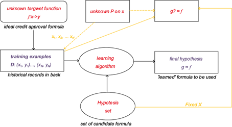
In recent years, machine learning has been proven to have a wide range of uses in engineering (e.g., in finance, manufacturing, and retail); nevertheless, it is steadily developing and being introduced into new fields (Khaled and Abdullah, 2016; Doreswamy et al., 2020). At present, the most widely applied machine learning methods include algorithms like the SVM, KNN, and the random forest. The process of machine learning can be summarized as follows: the collected training data are input, all possible hypotheses (expressed as functions) are tested using the learned algorithm, and the hypothesis which is closer to the actual pattern is identified (Liu et al., 2019, 2020, 2021). This same process is shown in Figure 1.
2.3 Deep learning methods
2.3.1 Recurrent Neural Network (RNN)
RNN is a type of recursive neural network which takes sequence data as input and carries out recursions in the direction of the series, with all nodes (i.e., recurrent units) connected in a chain (Feng et al., 2019; Tong et al., 2019). Its network architecture is shown in Figure 2.
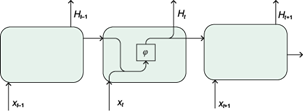
The input data were considered to be temporally correlated; moreover, we assumed that X
t
where φ represents the fully connected layer with the activation function. Through the previous process, the hidden variable H t-1 at the previous time step was saved and a new weight parameter was introduced to describe how the hidden variable of the previous time step was used at the current time step. Specifically, the calculation of the hidden variable at time step t was done based on both the input at the current time step and the hidden variable at the previous time step. The H t-1 W hh term was addedhere. From the relationship between the hidden variables H t and H t-1 at adjacent time steps in the above equation, it was found that the hidden variable can capture the historical information of the sequence at the current time step. This historical information reflects the state or memory of the neural network at the current time step; therefore, the mentioned hidden variable is also called hidden state. Since the definition of the hidden state at the current time step includes the hidden state at the previous time step, the calculation of the above equation was recurrent. A network with recurrent calculations is called an RNN. Such networks have usually the following activation function:
2.3.2 Long short-term memory (LSTM)
LSTM is a type of temporal RNN, which was specially designed to solve the long-term dependency problem of general RNNs (Graves and Schmidhuber, 2005; Yue et al., 2020). All RNNs are structured as chains consisting of repeating neural network modules. The network architecture of the LSTM is shown in Figure 3.
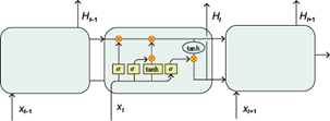
An LSTM has the ability to remove or add information to the cell state through carefully designed structures called gates. Each of these structures can selectively pass information; moreover, it contains a sigmoid neural network layer and a pointwise multiplication operator. The LSTM features three gates that are employed to protect and control the cell state. In particular, the forget gate determines what information is discarded from the cell state. Since the output of the sigmoid function is a value < 1, it is equivalent to a value reduction in each dimension. The input gate determines which new information is added to the cell state; meanwhile, the output gate determines which part of the cell state should be exported through the sigmoid.
2.3.3 Gated recurrent unit (GRU)
In order to overcome the inadequacy of RNN in handling long-range dependencies, we proposed the use of an LSTM. A GRU is a variant of the LSTM described above; notably, it is able to preserve the performance of the LSTM, although it is based on a simple structure (Tao et al., 2019). The network architecture of the GRU is illustrated in Figure 4.

From the network architecture diagram, it can be seen that the GRU obtains the states of the two gates from the last transmitted state H t-1 and the input of the current time step X t . As shown in Figure 4, r t controls the reset gate, which is expressed by the following equation:
z t is the update gate, which can be expressed as follows:
where σ is the sigmoid function. Using the function in Eq. (5), data can be transformed into values between 0 and 1 and hence used as gating signals. After obtaining the gating signals, the reset gate can be used to obtain the data after the reset. The reset process is expressed by Eq. (6):
The tanh activation function is mainly used to scale the data to values between -1 and 1. Here, h᷃ t mainly includes the current input data of X t and is added to the current hidden state in a targeted manner. This is equivalent to the memorization of the current state.
Finally, the GRU network performs the forgetting and memorizing steps simultaneously by using the previously obtained update gate z t . The updating process is expressed by Eq. (7):
The gating signals (i.e., z t ) range between 0 and 1. The closer the gating signal gets to 1, the more data are memorized; meanwhile, the closer it gets to 0, the more data are forgotten. Notably, GRU can simultaneously forget and select memory using only gate z t . The output of the final output layer is expressed by Eq. (8):
Data processing, experimental design, and evaluation
3.1 Data processing
3.1.1 Data overview
In this study, we mainly used relative humidity and visibility data obtained from the Shiyan Observation Base in Shenzhen metropolis between January 1, 2018 and August 31, 2019, as well as the data from the meteorological tower. Though haze is actually closely related to air quality and the Shiyan base does have some observational data on air quality, air quality data is not used in the current study. This is because most weather stations with visibility observations in Shenzhen do not have air quality observational instruments. On the other hand, the purpose of this study is to find appropriate machine learning methods to predict visibility for practical purposes. Therefore, adding air quality data to the current study is not helpful for obtaining a valid conclusion for all weather stations, especially those without air quality observations.
The observation base is located on the east bank of the Pearl River Estuary, about 10 km from the coastline. The visibility data collected from this base between May 2018 and July 2018 were missing and hence replaced by the visibility data collected in the Tiegang Reservoir (around Shiyan base). The sites of Shiyan and Tiegang are actually close to each other (around 5 km apart). By using a dataset with duration of one week from the two stations, it can be found that the correlation coefficient of the data between the two stations exceeds 0.98, and the relative error is less than 5%. The data structure is shown in Table I. All the observation equipment of Shiyan base is calibrated quarterly according to the operational management regulations. Moreover, quality control of the data has been performed and outliers have been deleted before they are used in the current study.
3.1.2 Data pre-processing:
Wind speed and direction, temperature, and humidity data collected continuously from the meteorological tower were processed as follows, creating a secondary processed dataset for the preparation of the training in the following step:
Average wind speed: the average value of wind speed between heights of 10-350 m.
Average wind direction: the average value of wind direction between heights of 10-350 m.
Average temperature: the average value of temperature between heights of 10-350 m.
Average humidity: the average value of humidity between heights of 10-350 m.
The data cycle was 10 min of the monitoring data. The data were normalized where needed and then divided into two subsets: the training and testing data set. Of all data, 80% were used as training data, which included all 2018 data, and the remaining 20% as testing data, which included the data for the first quarter of 2019.
3.2 Experimental design
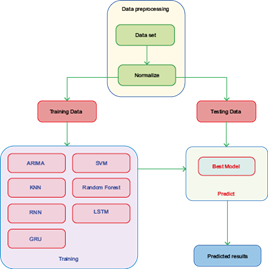
The flowchart of the experiment is shown in Figure 5. The test data is divided into two parts after data normalization. One part is used for training and the other part is used for prediction and verification. Once an optimal method is obtained through the training data, the prediction data will be used to verify the capability of the method.
3.3 Evaluation of the results
3.3.1 Root-mean-square error (RMSE)
The RMSE is the square root of the sum of squares of the deviation between the observed and true values and the reciprocal of the number of observations (m). This parameter can be used to measure the deviation between the observed and true values. If y̑ (test) represents the predicted value of the model in the testing set, then the RMSE can be expressed as
Intuitively, the error drops to 0 when y̑ (test) = y (test) . Moreover,
Therefore, when the Euclidean distance between the predicted and target values increases, the error also increases.
3.3.2 Mean absolute error
The mean absolute error is the average value of the absolute error, which can better reflect the actual error of the predicted value. If y̑ (test) represents the predicted value of the model in the testing set, then the mean absolute error can be expressed as
Intuitively, the error drops to 0 when y̑ (test) = y (test) .
3.3.3 Mean absolute percentage error
The mean absolute percentage error can not only consider the error between the predicted and true values, but also the ratio of the error to the true value. Thus, the mean absolute percentage error was used for evaluating the results. The mean absolute percentage error can be expressed as:
4. Analysis of the results
4.1 Factor analysis
Figure 6 shows a small part of the 10-min visibility forecast obtained by using humidity, temperature, wind direction, wind speed, and visibility data as input data. The forecasting results show that the wind speed was the physical parameter which best reflected the trends in visibility (besides visibility itself), followed by relative humidity; however, the forecast error was relatively large for the values of future visibility. It was difficult to predict the results of future visibility merely from temperature and wind direction; on the contrary, it was possible to accurately predict visibility at the next moment from that in the previous moment. Table II shows that the error can be further reduced by adding all factors.
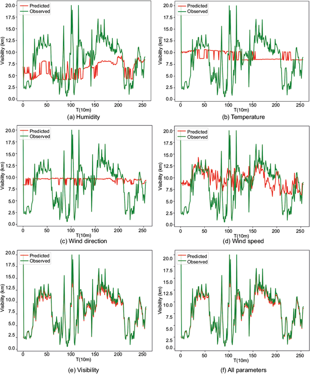
Fig. 6 Forecasting performances obtained by using different meteorological parameters and visibility.
4.2 Visibility forecasting performance
In order to compare the advantages and disadvantages of different statistical forecasting methods, we applied the seven methods mentioned in Figure 5 to forecast the visibility in the following 1, 3, 6, 24 and 72 h. The forecasts with different lead time have different functions. For example, the visibility forecast with lead time of 1 to 6 h is of great significance for real-time public traffic dispatching and guidance, while the forecast with lead time of 24-72 h could play a supporting role in longer-term traffic management and pollution source control. By comparing and analyzing the RMSE, MAE, and MAPE statistics of the forecast and actual results, we could determine the most suitable methods for visibility forecasting. In view of the results described in section 4.1, all the physical quantities relative to the previous time step were used for the forecasting of the next time-step data in all seven methods.
The forecasting performances of the seven models are compared in Figure 7, whose left column shows the performances of all seven models while the right column only shows the best one. Table III compares the MAPE of different methods for all forecast experiments, from which the performance of different models can be understood.

Fig. 7 Comparison of forecasting performances by using different models. The left column is for all seven models and the right column for the best one
Table III MAPE of different methods for all forecast experiments (%).
| Lead time | 1 h | 3 h | 6 h | 24 h | 72 h |
| ARIMA | 18.55 | -- | -- | -- | -- |
| SVM | 5.22 | 4.73 | 5.39 | 4.70 | 5.49* |
| KNN | 7.27 | 9.46 | 10.97 | 9.75 | 14.8 |
| RT | 4.96 | 6.11 | 7.92 | 6.25 | 6.83 |
| RNN | 3.38 | 3.08 | 5.66 | 4.5* | 6.75 |
| LSTM | 3.12* | 2.99 | 5.62 | 6.87 | 11.6 |
| GRU | 3.5 | 2.91* | 5.43* | 4.83 | 9.12 |
*Best performance.
As shown in Figure 7a, b, the 1-h average visibility was forecasted using 12 000 training and 3000 testing data points, respectively. The data volume was relatively large. A good forecasting performance could be obtained by all methods except ARIMA, by which MAPE reached as high as 18.55% in the current study. Given the large errors associated with the ARIMA method compared with those of other methods, it will not be further discussed. In the dataset of 1-h average visibility, the best performance was achieved by the LSTM method, followed closely by RNN and GRU.
In order to learn the performance of the models used in longer lead time, forecast experiments of the 3- and 6-h average visibility were carried out. The 3-h forecast experiment dataset has 3840 training data points and 960 testing data points, while the 6-h dataset has 1760 training and 340 testing data points. In the two experiments, the best performances were achieved by the GRU method, followed closely by the RNN and LSTM methods, as shown in Figure 7c-f.
As can be seen in Figure 7g, h, a forecast of the 24-h average visibility was performed using 480 training and 120 testing data points. In this type of dataset, the best performance was achieved by the RNN method, although a similar performance was achieved by the GRU method. A slightly poor performance was observed instead with the LSTM method.
A visibility forecast with a lead time as long as 72-h was also performed using 112 training and 32 testing data points, respectively. Since the number of training datasets was relatively small, the best forecasting performance for this type of dataset was achieved by the SVM method, which provides promising results in case of small-sample time-series forecasting. Despite the deviation in the forecast of the absolute value of visibility, the SVM method could still forecast the trend changes.
5. Conclusions
In this study, the visibility forecasting performance of different machine learning methods was compared using visibility data collected in the Pearl River Delta (Shiyan) and observational data obtained from a meteorological tower. The performances of different methods in forecasting the average visibility after 1, 3, 6, 24, and 72 h were tested. The following conclusions were reached:
Satisfactory visibility forecasting results could be obtained using historical visibility data. By adding information such as wind speed, wind direction, temperature, and humidity, the forecast accuracy can be further enhanced. In the current study, the MAPE of the prediction could be reduced from 5.01 to 3.8%.
Among all meteorological parameters, wind speed was the best at reflecting the visibility change patterns. Though the MAPE obtained by using wind speed is not significantly lower than those obtained by using other parameters, the predicted variation trend obtained by using wind speed is closer to the observed visibility than that obtained by other parameters. Therefore, it can be considered the most important meteorological parameter for future visibility forecasts (apart from visibility itself).
When short-term visibility forecasts (i.e., 1, 3, and 6 h) were performed, the forecasting performances achieved by the time-series modeling methods (i.e., RNN, LSTM, and GRU) were comparable to each other, due to the use of a large training dataset.
When mid- and long-term visibility forecasts (i.e., of 24 and 72 h) were performed, a classical machine learning method (the SVM) could also provide very good forecasting results, due to the use of a small training data set.
The forecasting of visibility using machine learning methods could achieve a certain degree of accuracy even for long periods (e.g., of 72 h). As long as the method selected is suitable, machine learning methods can be practically applied to visibility forecasting, though there is not a universal best method. If only one model is allowed to be used, the RNN is suggested, since the average value of MAPE for all experiments is the smallest one.
Although the machine learning method can achieve satisfactory visibility prediction, the prediction of sudden changes in data trends still has great limitations. Future possible researches to improve the performance could be focused on the following aspects:
Decomposing the data, obtaining high- and low-frequency information of the data, and processing different frequency information in different ways to extract the mutation law information in the data.
Combining the numerical models and the machine learning methods to improve the accuracy of prediction.
Developing new time-series forecasting models to improve forecasting accuracy.

