


 nueva página del texto (beta)
 Inglés (pdf)
 Artículo en XML
 Referencias del artículo
 Enviar artículo por email
 Citado por SciELO
  Similares en
SciELO
Similares en
SciELO 
 Permalink
1. Introduction
Geophysical processes and their graphical representation are commonly elaborated through spatial modeling. When it comes to regions lacking information on environmental parameters or challenging to access, such as mountain areas, this strategy becomes a valuable tool that is increasingly used to represent the environmental elements involved (Melesse et al., 2007; Yusoff and Rindam, 2012). As Soto Molina and Delgado Granados (2020) point out, in mountainous environments, the lack of observatories for long-term monitoring of the climatological variables that determine the state of their ecosystems is very common; therefore, spatio-temporal modeling represents the only alternative for understanding the atmosphere-surface relationship and its evolution over time.
Mexico has two-thirds of mountainous relief, so most of its ecosystems are found in regions with rugged orography at altitudes ranging from 700 to more than 5000 meters above sea level (masl) (INEGI, 2017). This means that large parts of the studies on the diversity of species in mountainous ecosystems are limited to indicating the existence and quantifying their coverage (Price, 2007) without considering two main climatic factors that govern their quality of life: air temperature and precipitation. These elements are of central importance in ecosystem studies since, as Magaña et al. (2004) and Hernández et al. (2017) point out, no matter how minimal their variation can be, it promotes ecological imbalance and can compromise the species and the ecosystem in general.
The territory of the state of Veracruz has the greatest orographic contrast in the country; its relief starts from sea level to the highest peak in the nation (Citlaltepetl volcano, 5610 masl). The altitude difference of its territory favors analyzing the existence of great biodiversity (Márquez Ramírez and Márquez Ramírez, 2009; CONABIO, 2011). Another example of its contrasting relief is the state’s north part, where the mountains that make up the Sierra de Otontepec Ecological Reserve (RESO by its Spanish acronym) stand out from the flat and homogeneous landscape surrounding them. Due to this altitudinal gradient, RESO has different ecosystems, including some endemic species (SEDESMA, 2007). Therefore, from an environmental conservation perspective, RESO has high scientific relevance, and the studies conducted at the site acquire national and international interest. However, despite its high ecosystem value, RESO lacks climatic information that strengthens the knowledge about the presence, distribution, and spatio-temporal evolution of the species that inhabit the area.
To remedy the absence of climate information in the country, the Universidad Nacional Autónoma de México (UNAM by its Spanish acronym) designed the Atlas Climático Digital de México (ACDM by its Spanish acronym), which covers the entirety of its territory through estimation by reanalysis (Fernández-Eguiarte et al., 2012, 2015). Nevertheless, its estimate represents a general atmospheric state (Dee et al., 2011) without considering the factors that determine microclimates’ existence, which are very common in mountainous areas (Lembrechts et al., 2018). At the same time, its spatial resolution does not provide accurate information for microscale studies since the raster grid of monthly data is 9 x 9 km and the daily ones are 1.8 x 1.8 km. In turn, for the calculation of the entire country, the planetary mean value of the vertical temperature gradient was used, which, as verified, varies remarkably from one place to another (Soto Molina and Delgado Granados, 2020). Therefore, despite the scientific value of the ACDM, mountain regions are not favored with its estimates because their orography changes in extremely small areas, on the order of tens or hundreds of meters at best. This results in adjacent ridges and valleys having the same precipitation and temperature values, which is highly unlikely in real life.
The high ecological value of RESO requires accurately detailing the temperature and precipitation distribution at the site and analyzing the changes these variables have experienced over time. Therefore, this work is focused on modeling through GIS the climatic parameters that determine the quality of life of the species that inhabit it. These results are intended to strengthen future research in the area of interest. At the same time, a simple and valid option is proposed that provides spatio-temporal climatic information in mountain sites lacking climatological infrastructure. This method is expected to be applied in mountainous regions whose scientific interest requires precisely estimating their climatic conditions.
2. Materials and methods
2.1 Study zone
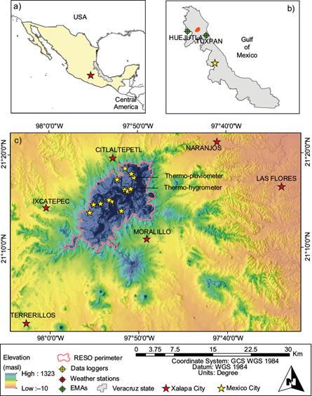
RESO is a mountainous set located in the Gulf’s North Coastal Plain, between the coordinates 21º19’19” and 21º09’34” north and 97º58’30” and 97º 48’00” west (SEDESMA, 2007) within the “Huasteca Veracruzana” region. In it, the municipalities of Ixcatepec, Tepetzintla, Chontla, Citlaltépetl, Tantima, Tancoco, Cerro Azul, and Chicontepec converge. It is located 230 km from Mexico City (the national capital) and 215 km from Xalapa, the state capital. The mountains that make up RESO stand out from the low and semi-flat territory surrounding them. Domínguez-Barradas et al. (2015) mention that despite its isolation, this area is a discontinuity of the “Sierra Madre Oriental” mountain range, one of the four mountainous provinces of the country. The characteristics of its relief, based on the 15-meter resolution DEM (INEGI, 2013), indicate that the delimitation of its perimeter is located at a minimum altitude of 310 masl and culminates at the summit of “Cerro Crustepec” at 1323 masl (21º14’24” north, 97º53’24” west); its origin is dated in the Cenozoic (SGM, 2004). The bedrock is composed entirely of basalt-type extrusive igneous rock; Robin (1976)) mentions that this basement is caused by lava emanation, the product of non-explosive volcanic eruptions. At least six geological faults are crossing the area in a north-south direction; these faults are likely associated with the eruptive activity that gave rise to them. The soils mainly comprise cambisols (INEGI, 1983) with a high organic matter content in the middle and upper parts.
It has a tropical (Aw2) or warm climate, the most humid of the sub-humid climates (Soto et al. 2001). However, its relief causes it to be modified by altitude and by the upward forcing of air masses. In the upper part, it is semi-warm humid (A)C(fm) with an annual average temperatures of 18 to 22ºC with an accumulated rainfall of ~1400 mm per year (García, 2004). The watershed formed by its summit separates the Tuxpan River basin to the southeast and the Panuco River basin to the west. Intermittent watercourses predominate in RESO that function as tributaries of perennial currents downstream. Figure 1 indicates the relative location of the study area.
2.2 Data and processing
To record the air temperature, 14 Hobo Pendant UA-001-64 data loggers were installed and programmed to store the data every 10 minutes for an entire year; one of these sensors had an additional Hobo MX2301 hygrometer to record the level of humidity in a mesophilic forest area. When the relief conditions allowed it, it was attempted to install sensors in the four slopes of the RESO, distributed in three elevation levels per side. Their altitudes were placed at 400, 700, and 1000 masl. A Hobo Rain Gauge RG3-M was placed at the top of the mountain to record the accumulated precipitation per event. All the sensors were factory calibrated with new batteries and synchronized simultaneously to homologate the data recording. The records were continuously and uninterruptedly collected from January 1 to December 31, 2020. Figure 1 (c) shows the position of the installed sensors and the weather stations used for reference.
The quality of the data obtained was verified by exploratory analysis in search of inconsistencies or atypical values, considering that the maximum temperature values were greater than those of the minimum ones, and the precipitation data were equal to or greater than zero. Because the data recording and storage were not interrupted and the sensors were always in the same place, it was considered that the series were homogeneous (Firat et al., 2012), always representing the weather conditions (WMO, 2011).
Data were tabulated and arranged chronologically. The vertical temperature gradient in RESO was obtained between the average temperatures of each of the three altitudes. This thermal gradient was calculated using the altitude differences and their corresponding temperature value between the three altitude levels. On the other hand, because the orographic rain in the Mexican mountains increases with the altitude up to the level of ~ 1800 masl, where the drying ratio begins with a negative gradient to the highest peaks of the country (Soto et al., 2020), the orographic rainfall gradient of RESO was obtained between the records of the rain gauge and those corresponding to Tuxpan and Huejutla automatic meteorological stations (EMAs by its Spanish acronym), whose data were obtained directly from the Servicio Meteorológico Nacional (SMN by its Spanish acronym) of the Comisión Nacional del Agua (CONAGUA by its Spanish acronym). Because both EMAs and the rain gauge automatically recorded the data every 10 minutes, this allowed comparing the precipitation regimes for each event simultaneously between RESO and the surrounding. Therefore, the precipitation gradient was also obtained from the difference between the recorded values and their altitude between the EMAs and the rain gauge, for a given event and at the same moment. Special care was taken to corroborate that the result was within the range indicated by Soto et al. (2020). Both gradients were used to distribute the temperature and precipitation values throughout the RESO mountain area.
Records obtained from the data loggers (temperature and precipitation) were correlated with the records of the weather stations around the mountain. The stations’ data was obtained from the main webpage of the Climate Computing Project (CLICOM). Special care was taken in the quality of the data from the stations used based on the WMO (2011) criteria. In addition to the homogeneity of the series, it was checked that the extreme values were within a maximum of four times the standard deviation value (Esteban-Vea et al., 2012; Soto Molina et al., 2019). The stations’ data averages a 38-year period, which allows for determining the climatological normal of a site or region (WMO, 1989; WMO, 2017). Table I shows the stations used. Based on the methodology of Soto Molina and Delgado Granados (2020), the gradients calculated in RESO were used to adjust the data of the selected stations in relation to the mountain relief.
Table I Weather stations around the study zone. Those marked with an asterisk correspond to the EMAs.
| Weather stations | 1981-2010 Annual Climate Normal | ||||
| Name | Altitude masl | Longitude | Latitude | Average Temperature ºC | Accumulated Precipitation mm |
| Ixcatepec | 173 | -98.00333º | 21.23944º | 23.9 | 1106.7 |
| Citlaltépetl | 220 | -97.87749º | 21.32916º | 23.9 | 1708.4 |
| Naranjos | 60 | -97.68166º | 21.35388º | 25.1 | 1313.5 |
| Las Flores | 50 | -97.56000º | 21.27583º | 24.0 | 1272.0 |
| Moralillo | 185 | -97.81400º | 21.18399º | 24.2 | 1134.6 |
| Terrerillos | 138 | -98.04111º | 21.03805º | 23.8 | 1378.8 |
| Tuxpan* | 7 | -97.41722º | 20.95972º | 25.8 | 1355.6 |
| Huejutla* | 115 | -98.36861º | 21.15472º | 23.6 | 1463.7 |
Because the stations used are located at different altitudes, the data adjustment procedure for each station and the subsequent modeling of the precipitation and temperature variables on RESO required standardizing the data at an altitude in common. In this case, the data were adjusted to sea level using the equation adapted from Fries et al. (2012) and Soto Molina and Delgado Granados (2020):
Where:
T x,y and P x,y |
Represent the value of temperature and precipitation corrected at sea level respectively |
T WS and P WS |
Is the real average temperature and precipitation of each weather station respectively |
Γ |
Is the gradient of temperature or precipitation in RESO |
Z Cor |
Is the altitude at which the conversion will be made, in this case it is 0 |
Z WS |
Is the real altitude of each weather station |
With the temperature and precipitation data adjusted to sea level, they were interpolated using the inverse distance weighted method (IDW), widely used in climatological variables (Kim et al., 2010; Rojas et al., 2010; Dobesch et al., 2013; Rodríguez et al., 2013; Yuan et al., 2016). This procedure yielded an interpolated layer per variable that covered the entire study zone as a flat or two-dimensional layer, delimited at the ends by the weather stations used. The interpolation made between the data from the stations around the mountain also included the data from the sensors installed on the slopes to make the modeling as real as possible according to the conditions determined by the terrain. This interpolation procedure was performed for each of the periods of interest; that is, the winter, summer, and annual average temperatures were interpolated; for its part, the interpolation of precipitation was for the rainy and dry seasons, and the annual accumulated.
The three-dimensional modeling of the climatological variables, distributed and adjusted according to the altitude of the relief, was carried out using the previously obtained interpolation layers and a DEM with a resolution of 15 meters per pixel (MPP). The DEM was obtained from the Instituto Nacional de Estadística y Geografía (INEGI by its Spanish acronym) main webpage. Therefore, the final layers of the three-dimensional climate modeling had a spatial resolution of 15 MPP, which allows any element, species, or wildlife population within each pixel to be analyzed with a good level of detail. The 3D climatological cartography of the RESO was obtained by using the formula adapted from Soto Molina and Delgado Granados (2020):
Where:
T x,y and P x,y |
Represent the value of temperature or precipitation at a point (x, y) respectively |
T Cor I and P Cor I |
Is the temperature or precipitation corrected at sea level, interpolated between the surrounding stations for any period of interest respectively |
Γ |
Is the temperature or precipitation gradient in RESO |
|
Is the value in altitude of a point (x, y) in a Digital Elevation Model, and |
Z Cor |
Is the altitude at sea level |
The above procedures were performed to estimate the air temperature during the summer and winter periods and for the annual average. The rainy and dry seasons (June-November and December-May, respectively) were calculated for precipitation and the accumulated annual total precipitation. From the complete interpolation layers between the surrounding stations and for each period, the final raster layers (final 3D maps) corresponding to RESO were extracted, limited by RESO’s perimeter.
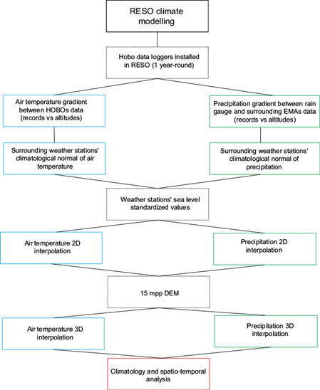
Finally, with the historical data from the surrounding weather stations, climate variability scenarios were modeled in RESO. The climate normals corresponding to the period 1981-2010 were analyzed considering that the standard climatological normals of any place on the planet are calculated in periods of 30 years, beginning at the first year of each corresponding decade (WMO, 2017), and that the data of the conventional stations cover on average from 1980 to 2016. To compare the variation in temperature and precipitation in the study area within the last 30 years, the averages of the two extreme ranges of the analysis period were compared, corresponding to the first and last decade (1981-1990 and 2001 -2010). Thus, considering that the main way to study temperature changes over time in mountain areas is through the altitudinal change of a reference isotherm (Soto Molina and Delgado Granados, 2020; Soto Molina et al., 2021), the altitude of the most representative isotherm and with the same value for each of the two periods was compared. Regarding the variable of precipitation, and as in the case of temperature, the averages of the decades 1981-1990 and 2001-2010 were also compared. Therefore, it was possible to identify the spatio-temporal variation of the accumulated annual total precipitation in RESO. Figure 2 shows the flow chart of the methodology described above.
2.3 Model Validation
For the model validation, temperature and precipitation data from climatological stations not considered during the modeling and were as close as possible to the study area were used. Considering that RESO is a small mountainous environment that stands out from the Gulf Coastal Plain, where the stations around it and the closest ones are at an altitude lower than 50 masl, it was necessary to resort to stations installed in mountain relief, located at an average distance of 165 km from RESO summit. In total, 13 stations, located at different altitudes from each other, were selected within RESO’s lower and upper limits.
As in the case of modeling, the 1981-2010 climatological normals of temperature and precipitation were used. The altitude values and the climatological normals were averaged from the group of stations. Subsequently, from the DEM of RESO, the isohypse with the same value as the altitude average of the group was obtained. Using the ArcGIS “intersect” tool, the values of the annual average temperatures and accumulated annual total precipitation were obtained for each pixel where the isohypse crossed to compare them with the average data of the group of stations. Finally, to further facilitate comparison, it was necessary to standardize the temperature and precipitation values at sea level, both for the stations and for RESO isohypse; the adjustment was made through the gradients used for modeling. Confidence intervals (CIs) were obtained from the values of the adjusted variables using the Student’s t-test (α = 0.95). Considering that the CIs in climatology are a helpful resource for the identification of similar climates (Mudelsse, 2014; Bowers and Tung, 2018), and due to the existence of different microclimates in each region, if the values of temperature and precipitation extracted from the isohypse of RESO were within the CIs determined by the group of stations, they would represent similarity conditions with a confidence level of 95%.
3. Results and discussion
The Gradients obtained in RESO were for the temperature, -0.0065ºC/m, and for the precipitation, 0.7 mm/m. With these gradients and the application of Eq. (1) and Eq. (2), the corresponding values adjusted at sea level were obtained for the summer and winter seasons, for temperature, and rainy and dry periods, for precipitation, along with the annual of both variables. Results are shown in table II.
Table II Temperature and precipitation adjusted at sea level per season.
| Weather station | 1981-2010 Temperature Climate Normal ºC (Sea level corrected) | 1981-2010 Precipitation Climate Normal mm (Sea level corrected) | ||||
| Name | Summer | Winter | Annual | Rainy season | Dry season | Annual |
| Ixcatepec | 28.22 | 20.59 | 25.02 | 724.8 | 153.52 | 878.4 |
| Citlaltépetl | 29.13 | 20.10 | 25.33 | 1152.8 | 265.2 | 1418.0 |
| Naranjos | 27.92 | 21.86 | 25.49 | 983.1 | 251.2 | 1234.3 |
| Las Flores | 27.90 | 19.46 | 24.33 | 971.9 | 234.1 | 1206.0 |
| Moralillo | 28.17 | 21.87 | 25.40 | 804.4 | 86.0 | 890.4 |
| Terrerillos | 28.23 | 19.57 | 24.70 | 996.0 | 201.6 | 1197.6 |
3.1 Temperature modeling
With the interpolation of the data corrected at sea level and with the use of the ArcGIS 10.5 Map Algebra toolset, in which Eq. (3) was introduced, the distribution maps of the average air temperature were obtained for the summer, winter, and annual periods in relation to the relief from the DEM. The sequence of figures 3 to 5 shows the geographical distribution of the normal average air temperature during summer (Fig. 3), winter (Fig. 4), and annually (Fig. 5).
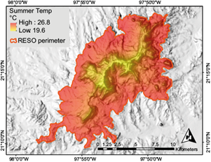
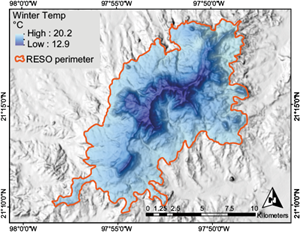
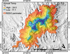
In the summer, the average air temperature value ranges from 26.8ºC in the lowest part of RESO (310 masl) to 19.6ºC at its top (1323 masl). However, it is within the limits of the northeast region, where the highest temperature exists. For its part, winter temperatures range from 20.2 to 12.9ºC, with the northeastern area showing the maximum value. Finally, annual average temperatures are distributed from 24.0 to 17.1ºC in the highest elevation.
Remarkably, for all periods, the northeast region is the one that shows the maximum temperature values. Likely, the orientation of RESO and the proximity of this area to the coastline favor the entry of warm and humid air from the Gulf of Mexico, particularly from the trade winds, influencing and affecting this area mainly. This situation can be corroborated by the annual wind direction diagram obtained with the Tuxpan EMA records (Fig. 6), which indicates that in 35% of the cases, the wind comes from the NE, followed by 25% from the N and 19% from E.

This situation is consistent with the findings of Perea-Moreno et al. (2020), who highlight that between the city of Poza Rica and the “Laguna de Tamiahua,” a wide region surrounding RESO, the wind has a prevalence from the NE and E during the year, being even more evident during the summer, when, also having high temperature, they transport a high oceanic moisture content. Likewise, this pattern of incidence of easterly and north-easterly winds is emphasized by Thomas et al. (2021).
The thermal ranges from the bottom to the top are very similar in the three periods: 7.2ºC for summer, 7.3ºC in winter, and 6.9ºC as annual thermal amplitude in relation to orography. This suggests that, except for the effect of continentality in the northeast, the horizontal and vertical temperature distribution shows a somewhat regular pattern; this must be a consequence of the thermal gradient obtained in the area (-0.0065ºC/m), which coincides very closely with the most common value in the country, according to Soto Molina and Delgado Granados (2020).
The conditions of temperature throughout the year show a relative similarity with the values indicated by García (2004). Nevertheless, the difference between the 18.0 to 22.0 ºC suggested by the author versus the 17.1 to 24.0 ºC obtained in this work is because García (2004) made her estimates with information from the stations close to RESO without considering the vertical variation of the variable. This situation highlights the need to calculate the specific thermal gradient of a study area when it comes to detailed research on ecosystems, especially when the climate determines their presence and quality of life.
3.2 Precipitation modeling
As with the case of temperature, figures 7 to 9 indicate the geographical distribution of precipitation in three seasons obtained from Eq. (4). Figure 7 corresponds to the rainy season, while the dry season is shown in figure 8; finally, figure 9 indicates the accumulated annual total precipitation.
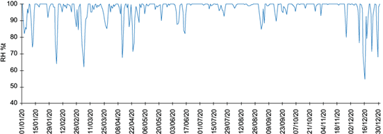
During the rainy season, an accumulated rainfall regime ranges from 1033 to 1820.1 mm (Fig. 7). As expected, the relief causes the upward forcing of the air and generates its consequent adiabatic cooling and condensation, which determines the highest concentration of precipitation in the highest parts of the mountain, as pointed out by Soto et al. (2020). However, the northeast region of RESO has a higher concentration of rainfall, contrary to the southwest area. On the other hand, the dry season (Fig. 8) shows a concentration ranging from 333.2 to 1049.5 mm. In the image, it’s possible to see that despite the low precipitation rate in the lower areas, the northern region concentrates more precipitation than the rest. This must be a consequence of the frequent arrival of northerly cold air masses from September to March, as pointed out by Jáuregui Ostod (1975), which coincides with the dry season in the country. These northerly winds (also known as northers) tend to discharge their humidity on the north and northeast slopes in response to the mountain's orography. Finally, the total accumulated precipitation per year (Fig. 9) indicates a concentration that ranges from 1183.5 mm in the lowest part of RESO and reaches 2070.9 mm in the highest part of the mountain. As in the case of the thermal variable, a more significant impact is observed per year in the northeast zone, contrasting with the opposite region that registers the lowest accumulation rate. This high level of humidity in the site can be observed through the records of the thermo-hygrometer installed in the north-eastern of RESO (as seen in Fig. 1), inside an area of cloud forest, at coordinates 21.2738º N, 97.8428º W. It can be noticed that the air remains mostly saturated during the months of June to November, while from December to May, the dry months, despite registering lower values of relative humidity (RH), are greater than 60%, being mostly between 80 and 100% of RH; conditioning an annual average RH of 96.4% (Fig. 10).
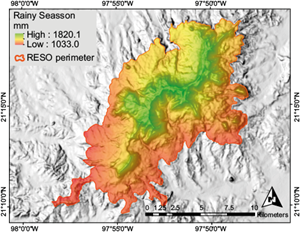
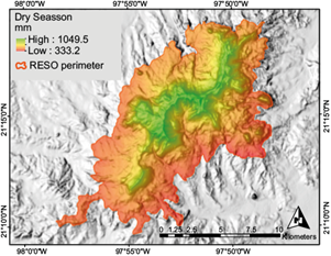
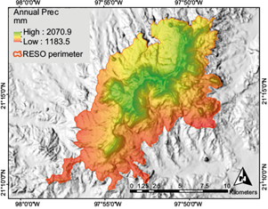
Interestingly, temperature and precipitation show higher values in the northeast region of the study area. It seems that the wind factor, both trade winds and the northers is responsible for this behavior in both variables. The above causes the RESO to have two somewhat different scenarios in climate or two distinct microclimates: the first being a warmer and more humid region in the northeast and another less warm but drier in the southwest.
The climatic conditions determined in this work govern the presence of native vegetation in RESO that is distributed as a function of the altitudinal gradient. It is essential to mention that Soto et al. (2022) identified the extensive presence of mountain mesophilic forest (MMF) in the highest parts of the north and northeast slopes of the study area. As is known, this ecosystem requires high atmospheric humidity conditions and a semi-warm to temperate air temperature, as indicated by Hinkle et al. (1993) and Ortega-Escalona and Castillo-Campos (1996)). Therefore, the presence of MMF in the study area coincides with the temperature and precipitation ranges identified in this work. On the other hand, the oak forest, and the tropical forest, located in the middle and lower parts of RESO (SEDESMA, 2007), are distributed according to a higher degree of temperature and lower precipitation, around 20ºC and 1600 mm as the mean value of precipitation per year, as mentioned by Santacruz and Espejel (2004). Both values have been notorious in this research below 1000 masl.
3.3 Climate variability
RESO shows changes in its climate patterns during the period 1981-2010. Based on figure 11, the average annual precipitation is observed in the decades 1981-1990 (Fig. 11a) and 2001-2010 (Fig. 11b). The reversal of the rainfall accumulation registered between the northeast and southwest regions is very noticeable, going from more to less rain concentration in the southwest zone. This decrease may be because between 1978 and 1988, according to Soto et al. (2020), the country was influenced by ENSO in its positive phase (ENSO+) mostly, which favored a higher income of humidity from the Pacific, generating greater increases of precipitation on the western slopes of the country. During the period 2001-2010, in which there was less humidity due to the presence of negative phases of ENSO (ENSO-) from 1999 to 2008, the intensity of the entry of the trade winds was re-established, giving rise to precipitation on the eastern and north-eastern slopes, decreasing at the same time on the western slopes. According to Folland et al. (1990), this type of pluvial variation pattern is prevalent in inter-tropical countries, where ENSO is the primary source of change in the rainfall regime.
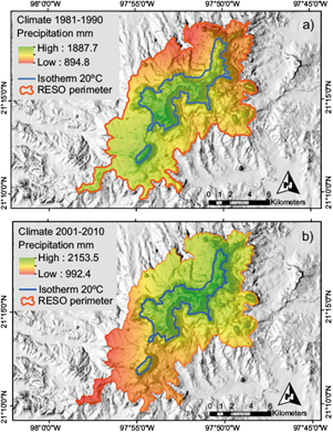
Fig. 11 Temporal changes in precipitation and temperature patterns for 1981-1990 (a) and 2001-2010 (b).
However, it is necessary to point out that the incidence of ENSO (+ or -) in the continental territory normally tends to be minimized as the distance to the Pacific coast increases; while it approaches the Gulf of Mexico shores, as in this case, this effect being minimized by the trade winds, as well as by tropical waves. Additionally, it should be mentioned that the properties of the relief influence the attenuation of its effects on the eastern region of the country, causing the moisture content coming from the Pacific to be forced to travel long distances, condensing and precipitating on the western slopes of the Sierra Madre Occidental and interior mountain ranges, due to the orographic forcing, during its displacement. These effects, the attenuation according to the distance from the Pacific (Magaña et al., 2003; Bravo-Cabrera et al., 2017) and the decrease in its impact on the rainfall regime due to orographic forcing, have been mentioned by Soto et al. (2020) in the Nevado de Toluca volcano, and are the causes of the relatively low degree of incidence in the precipitation of RESO.
Corroborating the spatial changes in precipitation described above, figure 12 is a composition from the reanalysis model MERRA-2 M2TMNXFLX (GMAO, 2015), which shows the concentration of precipitation for the two decades of comparison. At the same time, it displays the graph for positive, negative, and neutral ENSO 3.4 events. For 1981-1990, the positive ENSO episodes favored greater increases of precipitation in the western region of RESO. Also, it can be noted that the coastal state of Michoacan shows the possible effect of humidity ingress from the Pacific. For the 2001-2010 decade, in which positive ENSO events decreased and at least three negative ENSO episodes were recorded, moisture from the Gulf of Mexico entered, concentrating the greatest increase of precipitation on the eastern slope of RESO.
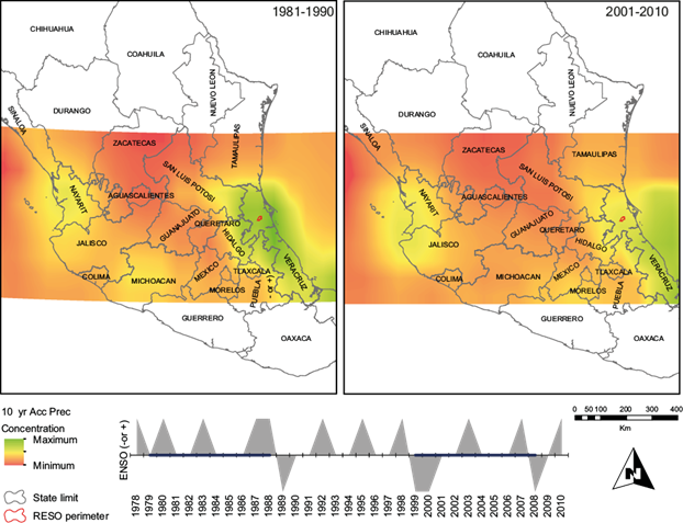
Fig. 12 Decadal model of reanalysis M2TMNXFLX for rainfall concentration in the country’s central region and graph of ENSO 3.4 events.
In accordance with the above and contrasting both periods of precipitation, four regions were obtained that show different degrees of variation. To determine these change zones, both periods were contrasted by the arithmetic difference between their raster layers. Four change categories were delimited and represented in an equal number of precipitation variation zones. Figure 13 (a) shows the areas from greatest to smallest decrease and from smallest to greatest increase in accumulated annual rainfall during the 1981-2010 period.
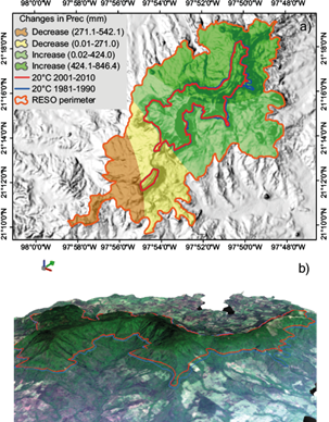
Fig. 13 Zoning of changes in precipitation between 1981 and 2010 (a). Image (b) shows an oblique RGB natural color view of RESO with the superposition of the 20ºC isotherms for the same period.
Probably, the variation of the rainfall regime in the extreme regions of RESO will continue as a product of the different phases of ENSO; therefore, its observation requires continuous monitoring of this phenomenon since, as in Central America and a large part of the Mexican territory, it directly influences the distribution and volume of precipitation.
Regarding the thermal variable, the isotherm of reference (20.0ºC) shows a change in its altitude that can be observed in figure 13 (a and b). According to the superposition of the isotherm with respect to the DEM, it has been possible to identify that it has ascended 18 m between the years 1981-2010, going from 790 to 808 masl, which represents an increase of 0.012ºC per year. Although this is a significant increase according to the IPCC (2018), it is a value lower than the ~ 0.2ºC that has been recorded on average on a global scale during the last decades (Hansen et al., 2006; IPCC, 2018; Zhang et al., 2020). Regardless of the degree of temperature increase registered in RESO, it is indisputable that its impact on the different ecosystems that inhabit it will cause them to experience its effects in the medium to long term; especially if the pluvial component is added, whose variation in spatial distribution and its quantity has been the product, among other factors, of the phases and degree of intensity of ENSO.
The temporal behavior of precipitation and temperature in RESO adjusts to the patterns that currently determine global climate variability since the pluvial variable shows spatial changes that can occur between years and decades, both in intensity and frequency, as indicated by Trenberth (2011), particularly in tropical regions. For its part, the temperature registers a more linear and homogeneous trend in terms of its gradual increase, as has been happening in all planet latitudes, as indicated by the IPCC (2018).
Regarding the values that were compared between the group of stations for validation and the model performance, the average values of the group of stations, at the same altitude, for temperature and precipitation, were 682 masl, 22.0 ºC, and 1718.2 mm, respectively. From the DEM of RESO, the isohypse 682 was obtained, through which the average temperature and annual precipitation values of 21.3 ºC and 1716.7 mm were extracted, respectively. This represents a difference of 0.7 ºC and 1.5 mm for each variable, respectively. Arithmetically the difference is minimal between the average of the group of stations and the isohypse of the model, which leads us to suppose, in principle, that the model results have an acceptable level of precision.
To corroborate the above, table III shows the values of temperature and precipitation adjusted to sea level. Their averages, standard deviation, and CIs were obtained from these values for the mean annual average temperatures (25.7ºC, 27.0ºC) and the accumulated annual precipitation (1006 mm, 1476 mm). The corresponding values of isohypse 682 corrected at sea level were 25.7ºC and 1239.3 mm, which are located within each CI. And according to Mudelsse (2014) and Bowers and Tung (2018), any value within the CIs represents a climate relatively similar to the group average with a probability of 95%.
Table III Group of stations for validation. Values for annual average temperature and annual accumulated precipitation.
| Weather station | Distance from the summit (km) | Direction | Altitude | Temperature (ºC) | Sea level corrected temperature | Precipitation (mm) | Sea level corrected precipitation |
| Huehuetla | 91 | SSW | 424 | 23.4 | 26.2 | 2397.9 | 2101.1 |
| Jalcomulco | 240 | SSE | 335 | 24.6 | 26.8 | 1080.5 | 846.0 |
| Tierra Blanca | 105 | W | 398 | 23.7 | 26.3 | 1800.6 | 1522.0 |
| Piedras Negras | 90 | S | 425 | 23.3 | 26.1 | 1452.7 | 1155.2 |
| Gallinas | 158 | WNW | 314 | 24 | 26.0 | 1552.9 | 1333.1 |
| San Dieguito | 162 | NW | 346 | 22.9 | 25.1 | 1364.7 | 1122.5 |
| Huautla | 50 | SW | 503 | 21.7 | 25.0 | 1327.4 | 975.3 |
| Damian Carmona | 173 | NW | 491 | 23.8 | 27.0 | 1519.8 | 1176.1 |
| Tamapatz | 133 | WNW | 1071 | 20.6 | 27.6 | 2571.1 | 1821.4 |
| Teocelo | 227 | SSE | 1188 | 20.6 | 28.3 | 2035.8 | 1204.2 |
| Cosautlan | 232 | SSE | 1274 | 19.9 | 28.2 | 2117.2 | 1225.4 |
| Rancho Viejo | 230 | SE | 914 | 20.5 | 26.4 | 1146.5 | 506.7 |
| Huatusco | 252 | SSE | 1186 | 17.2 | 24.9 | 1969.9 | 1139.7 |
| Average | 682 | 22.0 | 26.4 | 1718.2 | 1240.7 | ||
| StDev | 1.07 | 389.0 | |||||
DF: degrees of freedom; Adj SS: adjusted sum of squares; Adj MS: adjusted mean sum of squares; F-value: is the F-statistic; P-value: is the value of significance.
An additional test for the model accuracy was carried out by comparing the monthly records of 2020 between Tuxpan and Huejutla EMAs against three sensors (indicated by their serial number) installed in the upper part of the mountain at 1000 masl. Before spatial interpolation, the data were standardized at sea level for correct contrast. Figure 14 indicates a very homogeneous and similar behavior among the five-time series with similar values. This similarity was statistically corroborated using an ANOVA test, which indicates that with a p-value of 0.882 > 0.05, all the groups are significantly like each other. Likewise, the pooled standard deviation = 3.08 confirms that the data are homogeneous and are within the quality parameters according to the criteria of WMO (2011), Esteban-Vea et al. (2012), and Soto Molina et al. (2019) (table IV).
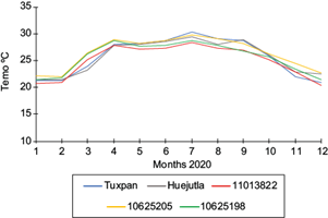
Fig. 14 Comparison of monthly values during 2020 between EMAs and temperature sensors installed at 1000 masl in RESO.
Table IV ANOVA for the five temperature groups compared.
| Analysis of Variance | ||||||
| Source | DF | Adj SS | Adj MS | F-Value | P-Value | |
| Station | 4 | 11.05 | 2.763 | 0.29 | 0.882 | |
| Error | 55 | 521.78 | 9.487 | |||
| Total | 59 | 532.83 | ||||
| Means | ||||||
| Station | Month-N | Mean | StDev | 95% CI | ||
| 10625198 | 12 | 25.619 | 2.810 | (23.837, 27.401) | ||
| 10625205 | 12 | 26.373 | 2.881 | (24.591, 28.154) | ||
| 11013822 | 12 | 25.019 | 2.985 | (23.237, 26.801) | ||
| Huejutla | 12 | 25.689 | 3.106 | (23.907, 27.471) | ||
| Tuxpan | 12 | 25.710 | 3.560 | (23.930, 27.490) | ||
Pooled StDev = 3.08007.
DF: degrees of freedom; Adj SS: adjusted sum of squares; Adj MS: adjusted mean sum of squares; F-value: is the F-statistic; P-value: is the value of significance.
Finally, it is essential to point out that the model’s precision level (tenths of a Celsius degree for temperature) is similar to that obtained by Soto Molina and Delgado Granados (2020). Even, despite being a simple and easy-to-replicate model, it presents better precision than more complex models, such as the one proposed by Yang et al. (2011), or the ACDM, since due to its low spatial resolution and the use of a single vertical temperature and precipitation gradient for the entire country, it generates considerable errors in its estimates. In addition to the above, our work highlights the ease of analyzing the evolution of the climate over time, which gives a valuable advantage to this work.
4. Conclusions
This work combines climatological analysis and the use of GIS technology. The climatic cartography elaborated for RESO, with in situ data and through the calculation of specific gradients of the study area, offers a level of precision that exceeds the climate models estimated by reanalysis carried out in the country. The pixel size (15 m) in the resulting raster maps obeys the relief patterns and facilitates the detailed analysis of any ecosystem element or population and its relationship with the climate that determines its existence, abundance, and distribution. Therefore, any ecological work carried out in the study area will be strengthened by correlating it with its surroundings’ climate to understand its current state and determine possible future scenarios.
RESO’s temperature and precipitation models adjust to the spatio-temporal behavior observed in intertropical zones, showing a spatial variation of rainfall and a gradual increase in air temperature over time. This work solves the lack of spatial-temporal information regarding the climate in mountainous areas, where the characteristics of the relief favor the existence of different ecosystems. Therefore, having an adequate model with a good precision level will help strengthen the studies of diverse ecosystems and their temporal evolution. Considering the methods and reasons for the elaboration of this work, it is expected that this cartographic modeling of climate will serve as a reference for regions of high ecological relevance where the lack of atmospheric data limits or prevents the investigations that intend to be carried out in the place.

