


 text new page (beta)
 English (pdf)
 Article in xml format
 Article references
 Send this article by e-mail
 Cited by SciELO
  Similars in
SciELO
Similars in
SciELO 
 Permalink
1. Introduction
Pollutants are monitored in many countries because of their risk to human health and environmental impact (SEMARNAT, 2013). Most are directly derived from combustion processes at fixed or mobile sources. The main criteria pollutants around the world are carbon monoxide (CO), sulfur dioxide (SO2), nitrogen dioxide (NO2), tropospheric ozone (O3), and particulate matter (PM) (Tyler et al., 2013). The health effects depend on exposure time and concentration (Mapoma et al., 2014). In 2012, the World Health Organization (WHO) estimated that one out of every nine deaths resulted from air pollution-related conditions (WHO, 2016).
Combustion processes are involved in the emission of most pollutants and increase the amount of gases in the atmosphere at different scales. In particular, SO2, NOx, and CO are generated by industrial activities and the burning of fossil fuels. The latter two also contribute to the formation of tropospheric ozone (O3) (Lazaridis, 2011) through photochemical reactions. This process depends on energy from solar radiation and is further exacerbated by increasing concentrations of NO2 and volatile organic compounds in the atmosphere (Sillman, 1999). It is important to analyze the interaction of these pollutants with meteorological parameters on a local scale.
Specifically, understanding the behavior or tendency of NO2 levels in urban areas is key for monitoring and mitigation strategies because of its relation with other pollutants and greenhouse gases (Gaffney and Marley, 2003). This knowledge, for example, has enabled the implementation of strategies to reduce emissions in several European cities (Henschel et al., 2015). On the other hand, in emerging cities and countries where industrial activities have increased in recent years, such as in Beijing, China, severe pollution warnings are emitted (Hou et al., 2016). In urban areas of Japan such as Tokyo and Osaka, a correlation was found between increasing NO2 concentrations and temperature, exacerbating heat islands (Gotoh, 1993).
The remote sensing of atmospheric NO2 and O3, among other atmospheric pollutants, can be performed using differential optical absorption spectroscopy (DOAS) (Platt and Stutz, 2008). In this technique, scattered light from the sun is carried onto a linear array-based spectrometer. Many measurement campaigns around the world have analyzed NO2 in the atmosphere using this technique, especially in large cities in Europe (Platt and Perner, 1980), China (Bernard et al. 2015), the United States (Spinei et al., 2015), and in several Latin American urban areas and volcanic regions (Grutter et al., 2008; Frins et al., 2011).
In Mexico City and its surroundings, the presence of NO2 has similarly been analyzed by spectroscopy techniques (Grutter et al., 2008, Melamed et al., 2009; Rivera, 2013). The DOAS technique has mostly been used in Mexico City to identify the vertical distribution of NO2 in the troposphere and its relationship with meteorological parameters such as wind speed and temperature (Melamed et al., 2009; Arellano et al., 2016). Atmospheric monitoring in Mexico City has been carried out since 1986, when the Red Automática de Monitoreo Atmosférico (Automatic Atmospheric Monitoring Network, RAMA) began to measure several pollutants (SEDEMA, 2017). The Sistema Nacional de Información de la Calidad del Aire (National Air Quality Information System, SINAICA) provides access to a database with data from every sensing station in Mexico (INECC, 2017). However, air quality has not been consistently monitored over the years. In this context, the use of atmospheric models to analyze the transport of pollutants and their interaction with meteorological events has been very useful to understand these realities. In Mexico City, local atmospheric conditions have been simulated by the WRF/Chem model, and a high correlation of meteorological parameters and NO2 was found when compared to observations (Zhang et al., 2009).
In 2008, 40% of NOx emissions in Mexico were estimated to come from mobile sources (SEMARNAT, 2013). The growth of cities has favored an increase in NO2 emissions. Measured emissions in 2013 and emissions projected to 2030 indicate that levels of this pollutant will continue to occupy the third place (9.84 × 10⁵ Mg year-1 in 2013 and 5.08 × 10⁵ Mg year-1 in 2030) behind CO (3.28 × 10⁶ Mg year-1 in 2013 and 2.16 × 10⁶ Mg year-1 in 2030) and CO2 (1.48 × 10⁸ Mg year-1 in 2013 and 2.47 × 10⁸ Mg year-1 in 2030) (INECC, 2014).
The measured atmospheric NO2 concentrations in several Mexican states are barely under the limit set by official Mexican standards. Although most large Mexican cities have an air quality monitoring system, the monitoring networks of several cities such as Guadalajara, Tabasco, and San Luis Potosí, among others, need to be updated due to maintenance problems and the quality of measurements according to a report carried out in 2009 (INE, 2011).
In particular, the municipality of San Luis Potosi has a high level of NOx emissions (18%), equaling 22 614.56 Mg in 2011 (SEGAM, 2013), largely due to vehicle combustion processes. In the span of 20 years (1990 to 2010), the population grew 32% (IMPLAN, 2016). At the same time, the vehicle density in the metropolitan zone of San Luis Potosí-Soledad de Graciano Sánchez increased 33% from 2005 to 2015 (INEGI, 2017).
The increase in vehicles and fossil-fuel-based industrial activities in the city of San Luis Potosí (INEGI, 2014) has correspondingly led to an increase in mobile and point sources of NO2. Therefore, the objective of the present study is to quantify NO2 in the atmosphere of San Luis Potosi using a spectroscopy technique and to analyze and explain its variability in relation to the behavior of several meteorological parameters obtained from the WRF model.
2. Methodology
2.1 Theoretical model
The DOAS technique (Noxon, 1975; Solomon and Schmeltekopf, 1987; Platt and Stutz, 2008) utilizes the structured absorption of many trace gases in the UV spectral region. It relies on the application of the Beer-Lambert law to the atmosphere considering a limited range of wavelengths. This law states that the radiant intensity traversing a homogeneous medium decreases exponentially with the product of the extinction coefficient, the number density and path length. The Beer-Lambert law applied to the atmosphere is written as follows (Danckaert et al., 2017):
where I(λ) is the measured spectrum after extinction in the atmosphere; I o (λ) is the spectrum at the top of the atmosphere, without extinction; σi(λ) (in cm2 molecule-1) is the absorption cross section of the i-th species, which is wavelength dependent; and c i (in cm2 molecule-2) is the column density of the i-th species defined by the concentration integrated along the light path in the atmosphere (Platt and Stutz, 2008).
From Eq. (1), we define the optical density as:
The basic idea of the DOAS technique is to separate the broad and narrow spectral structures of the measured spectra in order to isolate the narrow structures associated to the different chemical species contained in the atmosphere. To perform that procedure, it is necessary to know the absorption cross section of each species in the spectral range of interest (taken from literature) and fitting the measured spectra by using Eq. (2) and determine numerically the optical density and the column density of each species. In the procedure, we have assumed that the absorption cross sections are independent of temperature and pressure. Thus we use the concept of Slant Column Density (SCD) to refer to c i (Danckaert et al., 2017).
2.2 Experimental set-up and NO 2 measurement via DOAS
The telescope used to measure DOAS is composed by a lens with a 2.54-cm diameter and a focal length f = 50 mm coupled to an optical fiber with a diameter d = 1000 mm (Fig. 1). With these parameters, the field of view (FOV) of our instrument defined as d/f (Frins et al., 2006) gives a value of approximately 1.1º. The light captured by the optical fiber was guided to a digital UV-Vis lightweight spectrometer (B&W Tek, model BRC641E) with Czerny-Turner configuration and a one-dimensional charge-coupled device (CCD) array (2048 pixels) with a resolution of 0.3 nm full width at half maximum (FWHW) and a spectral range from 198 to 450 nm. The integration time was 100 ms to prevent saturation throughout the day. The acquisition program averages 100 spectra and saves the resultant spectrum. The system is cooled at constant temperature of 18 ºC by a thermoelectric regulator to minimize the dark current (Arellano et al., 2016).

To determine the NO2 composition, we have analyzed spectra in the range from 360 to 420 nm. In this region, the spectral composition of NO2 has been fully identified (Rublev et al., 2003). Two spectra were considered for DOAS analysis: one (reference spectrum) acquired at zenith (around noon) and the other measured also at zenith but temporarily displaced from the reference. The latter spectrum is normalized by dividing the reference spectrum in order to discriminate slow spectral information structures.
3. Data analysis
3.1 Study area
The City of San Luis Potosí is located in central northern Mexico (22º N, 100º W) at 1860 masl (INE, 2011). The prevailing climate is dry and semi-dry. The statewide average annual temperature is 21 ºC. The average minimum temperature is −5 ºC, occurring in January, and the average maximum temperature is around 38 ºC from May to July. The rainy season spans the summer from June to September, and the average precipitation is about 300 mm annually (Rivera, 2014).
From July to August 2015, a sampling campaign was carried out at the Instituto de Investigación en Comunicación Óptica (Research Institute for Optic Communications, IICO). In Figure 2, the locations of IICO and the meteorological station (northeast of the sampling point) are shown. Data from the meteorological station were used to validate the data obtained by using WRF. Subsequently, WRF was used to obtain the meteorological data at the IICO site where NO2 was measured.

3.2 Spectral analysis
The spectra were measured statically between 8:00 and 17:00 LT (UT-6). The electronic offset induced by the CCD dark current of our system was obtained by obstructing the light entrance of the spectrometer and measuring the output signal of the CCD array. This procedure was performed every day at the beginning of each set of measurements. The offset signal was numerically subtracted from the reference spectrum (taken at noon) and from every spectrum taken during the day. After that, the spectra were divided to normalize them. A low-pass filter was used to separate the broad and narrow spectral bands (Rivera et al., 2013). By using Eq. (1), the experiments and the cross-section of the gases of interest, we evaluated numerically the SCDs of each species.
The numerical approach was performed by using the QDOAS software (Danckaert et al., 2017) and high-resolution differential cross-sections in the spectral range from 360 to 420 nm of NO2 (Vandaele et al., 1998), O3 at 221 and 241 K (Burrows et al., 1999), oxygen dimer (O4) (Hermans et al., 1999) and a Ring spectrum generated at 273 K (Kurucz, 1995).
3.3 Urban atmospheric conditions generated by the WRF model
Atmospheric conditions were simulated by the WRF model due to the lack of meteorological data at the location of the experiment. The WRF model is a non-hydrostatic, numerical and three-dimensional model that uses sigma levels in physical equations to determine a vertical distribution in which the dynamic of the atmosphere is studied under different physical parameterization schemes (Skamarock et al., 2008). It was developed by Pennsylvania State University and the National Center for Atmospheric Research (NCAR), among others (Guichard et al., 2003; Skamarock et al., 2005). The global weather data fed to the model were obtained from the National Center for Environmental Prediction (NCEP) and had a spatial resolution of 100 × 100 km with time intervals of 6 h for every input variable considered (Kalnay et al., 1996).
Physical variables are also included in the WSM 6-class graupel scheme, such as condensation, precipitation, and latent heat (Lim and Hong, 2005). The Rapid Radiation Transfer Model (RRTM) was incorporated to consider the influence of long-wave radiation and the Dudhia (1989) scheme to consider the influence of short-wave radiation.
The model was calculated for three surfaces: the largest was 1500 × 1500 m, the other two were nested domains of 500 × 500 and 250 × 250 m. The experiment began on July 27, 2015 but the modeling was carried out from three days before (July 24) to stabilize the model. The simulation ended on August 16, 2015. Meteorological data were extracted from the WRF model for the same location where NO2 was measured (Fig. 2).
The analyzed parameters were solar radiation, temperature, wind speed, and relative humidity because of their importance in the creation and destruction of NO2, as emphasized by Pineda-Martínez et al. (2012).
The only place where a meteorological synoptic station (MSE) may be found is to the north of the city, for which the WRF results were validated in that location by comparing the meteorological data measured with those generated by the model. Subsequently, the NO2 levels measured south of the city were compared with the meteorological data calculated (Fig. 2) to analyze the relation between these parameters. The BIAS and root mean square error (RMSE), whose reliability was confirmed by Pineda-Martinez et al. (2012), 2014), were calculated.
4. Results and discussion
4.1 WRF simulations
Figure 3 shows some examples of the meteorological station data and the corresponding simulations obtained by WRF for wind speed, temperature, and relative humidity for July 31, July 29 and July 29, respectively. The model predicts well the general behavior for wind speed, temperature and relative humidity, respectively in the period from 8:00 to 13:00 LT. The modeling nested domain was carried out on a 250 × 250 m grid.
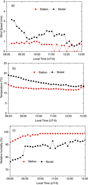
Fig. 3 Comparison between data from the meteorological station and data generated by the WRF model for: (a) wind speed on July 31, (b) temperature on July 29, and (c) relative humidity on July 29.
The statistical confidence of wind simulations decreases at resolutions lower than 3 km, especially for higher run periods (Pineda-Martínez et al., 2012). In this case, the reliability of the WRF model in predicting wind speed was highest on July 31, with a RMSE of 0.91 and a BIAS of −0.54 m s-1, whereas the lowest confidence was recorded on August 1, with a RMSE of 2.05 and a BIAS of −1.67 m s-1. It is difficult to analyze urban conditions at this resolution because, near the surface, there is influence from convective processes, turbulent effects of air flow, and buildings (Pineda-Martínez et al., 2014). The behavior of wind speed differed daily due to local conditions, whereas the behavior of temperature showed some common patterns.
Relative humidity explains the aforementioned case. For example, at almost the same time when temperature was underestimated by the model with respect to the meteorological station (13:00 h), relative humidity was overestimated (Fig. 3c). This could result from the influence of the mountains surrounding the urban area and the trade winds from the eastern Sierra Madre (Pineda-Martinez et al., 2014), causing a mountain breeze effect in the afternoon.
However, the model can explain meteorological behavior with good confidence in the morning until approximately 13:00 LT. After this time, the recorded relative humidity tended to decrease, while the recorded temperature tended to increase. The model, on the other hand, indicated water vapor saturation (high relative humidity reaching 100%) and temperature decrease (Fig. 3b, c).
4.2 NO 2 optical density
To illustrate the performance of the technique we show in Figure 4, optical density was obtained for: (a) NO2, (b) O3, (c) O4, and (d) the ring spectrum. The spectra were measured on August 1, 2015 at 10:52 LT, with 1-min time integration in the wavelength range from 360 to 420 nm. Black spectra are the contributions to the optical density of each species and the red lines are the fitted spectra. The numerical approach was obtained by using QDOAS software. We found that in this range the optical track of NO2 was well resolved. Note that the contribution of O3 and O4 in this range is not evident. The contribution of the ring spectrum (Fig. 4d) is clear and it is dominated by sharp structures below 400 nm. To have further evidence of the performance of our technique, we show in Figure 5 the contribution of O3 and O4 bands in the range from 340 to 370 nm, where the presence of these gases is evident.

Fig. 4 Optical activity measured on August 1, 2015 at 10:52 LT with 1-min time integration for (a) NO2, (b) O3, (c) O4, and (d) the ring spectrum for the wavelength range from 360 to 420 nm. Black lines are the spectra obtained numerically from the measured spectrum, the absorption cross section of the gases of interest and Eq. (2). The red lines are the fitted spectra. The numerical approach was obtained by using the QDOAS software.

4.3 NO 2 column behavior and interaction with meteorological parameters
Black circles in Figure 6 show the SCD of NO2 obtained by QDOAS on (a) July 28, (c) July 29, and (e) July 31 between 8:00 and 16:00 LT (UT-6). All the SCD curves increase their value during the first 2 h and reach their maximum at (a) 11:00, (c) 9:45 and (e) 9:30 LT. After that, the curves start to decrease. The maximum SCD value for each day is (a) 2.5 × 10¹⁶, (c) 2.0 × 10¹⁶ and (e) 2.1 × 10¹⁶ molecules cm-2. These SCD values of NO2 are below those measured at other cities: for example, in Mexico City, the NO2 column oscillates around 2.0 × 10¹⁷ molecules cm-2 according to the measurements of Rivera et al. (2013).

Fig. 6 SCD of NO2 measured on (a) July 28, (c) July 29, and (e) July 31, and relationship between wind speed and relative humidity estimated by WRF on (b) July 28, (d) July 29, and (f) July 31.
In order to correlate the SCD behavior with meteorological parameters, we also show in Figure 6 meteorological data generated by the WRF model for the same days and hours of the SCDs data. Figure 6 includes wind speed (blue triangles) and relative humidity (orange triangles). The highest values of the NO2 column (around 2.0 × 10¹⁶ molecules cm-2) were found around (a) 11:00, (c) 9:30 and (e) 9:00 LT. These peaks were possibly influenced by minimum wind speed around 9:30 LT, or by human activities.
The decrease of the NO2 column can also be associated to the increase of relative humidity during the day. The levels of concentration for air pollution depend on the levels of emissions but also meteorological conditions as wind speed, temperature, rainfall, and relative humidity, which have influence in the formation of secondary pollutants and atmospheric dispersion (Crutzen, 1979; Countess et al., 1981, Habeebullah et al., 2015).
5. Conclusions
The presence of NO2 in the atmosphere was characterized for the first time using remote sensing techniques (DOAS) in San Luis PotosÍ, Mexico. Additionally, meteorological data such as wind speed, relative humidity, and surface temperature were estimated by the WRF. The parameters estimated by the WRF model were reliable from 8.:00 to 12:30 lt. Later in the day, it was necessary to consider data from a meteorological station to describe the variability of NO2.
The highest sensitivity of the technique for the detection of NO2 was obtained for the wavelength range from 360 to 420 nm. The method utilized herein represents an alternative for monitoring atmospheric gases in the city of San Luis Potosí. It is suitable for understanding the distribution of gases at specific sites (based on surface measurements) as well as across regions. This method can be extended to analyze other gases such as SO2, O3, and BrO at different wavelengths in the UV rage.

