


 text new page (beta)
 English (pdf)
 Article in xml format
 Article references
 Send this article by e-mail
 Cited by SciELO
  Similars in
SciELO
Similars in
SciELO 
 Permalink
1. Introduction
Bahía de La Paz is a semi-enclosed body of water located on the western side of the Gulf of California (GC), near the southern end of the Baja California Peninsula (Fig. 1). It is ~80 km long by ~35 km wide, with a surface area ~2700 km2. The main bathymetric feature is in the northern part: the 450-m deep Alfonso basin, with a sill at 250-300 m at the main connection with the GC, between Punta Mechudo and the north tip of Espíritu Santo Island (Fig. 1). In the south of the bay, the narrow and shallow (< 18 m) San Lorenzo channel probably plays a minor role in the low-frequency interchange of waters between the GC and the bay.

Fig. 1 (a) Bahía de la Paz, with bathymetry (m). Stars indicate the positions of the oceanographic stations made during the NAME-II cruise. Line of stations L1-L7 is referred to in the text. (b) Wind velocity from ship data during cruise. (c) Map of the southern portion of the Baja California Peninsula with topography (m). The insert square shows the location of Bahía de la Paz.
Monreal-Gómez et al. (2001) found that during June 1998 the geostrophic circulation in the northern Bahía de La Paz was cyclonic, and suggested that it could be related to the wind curl. Salinas-González et al. (2003) found evidence of anticyclonic geostrophic circulation in October 1997 and August 1999. Sánchez-Velasco et al. (2006) found cyclonic circulation in July and October 2001, and weak undefined patterns of circulation in May 2001 and February 2002. The latter authors argued, based on fish larvae distributions, that the circulation inside the bay may be connected to the overall seasonal circulation of the GC. During August, 2009, the presence of a cyclonic eddy confined in the northern of Bahía de La Paz was also documented, implying their importance in the distribution of nutrients concentrations and different trophic groups of zooplankton in the region (Coria-Monter et al., 2014; Durán-Campos et al., 2015). The latter authors suggested that the eddy origin could be linked with the topography of the basin and the interaction of the current entering to the bay through Boca Grande (Fig. 1).
These works suggest that cyclonic circulation is a frequent summer feature of the bay’s geostrophic circulation, but that the anticyclonic pattern is also possible. However, geostrophic calculations can give only an approximation of the circulation; previous works have taken the bottom, 50 m, or base as level of no motion (to include as many stations as possible), while the distribution of thermohaline variables in vertical cross-sections of the summer hydrography suggest that the cyclonic circulation is at least 150 m deep (Durán-Campos et al., 2015).
The wind field over the GC changes direction with the seasons, blowing from the northwest during winter and from the southeast during summer (see, e.g., review by Lavín and Marinone, 2003; Marinone et al., 2004; Bordoni et al., 2004). The wind over the Bahía de La Paz bay shows the same pattern in winter and fall, however, during late spring and summer winds from southwestern component predominate (Herrera-Cervantes et al., 2017; Muñoz-Barbosa et al., 2020). I has been reported that Bahía de La Paz bay has a strong coupling between wind stress curl, sea surface temperature, and chlorophyll-a (Herrera-Cervantes, 2019).
In this work we present the first directly-observed description of the summer circulation in Bahía de La Paz, based on observations made during the summer of 2004, using satellite-tracked surface drifters and vertical Lowering Acoustic Doppler Current Profiler (LADCP) profiles. The consequences of the bay’s circulation on its surface temperature and chlorophyll are described by analysis of satellite data. The role of the wind stress curl on SST and productivity (CHL) of the bay is investigated using a time series of satellite-derived daily wind velocity.
2. Data and methods
Lagrangian surface currents were observed with two Pacific-Gyre SVP ARGOS drifters equipped with holey socks centered at 15 m (see Lavín et al., 2014). The first drifter (s/n 50021) was inside the bay from June 18 to July 18, 2004, and the second (s/n 52083) from August 16 to October 11, 2004. The drifters transmitted their positions in average every 3 h, with accuracy ~300 m, which resulted in an observed velocity error of ~0.028 m s-1. We performed a linear interpolation to obtain positions exactly every 3 h, from which velocities were computed.
One 17-day campaign (NAME-II) was made from the research vessel Francisco de Ulloa, from August 6 to August 22, 2004, covering most of the southern GC (Lavín et al., 2013), but for this paper we use only data collected between August 15 and August 16 inside Bahía de La Paz (Fig. 1). The spacing between stations was ~10 km in the across-bay transects, and the distance between transects was ~25 km. The thermohaline profiles to ~3 m above the bottom were measured with a factory-calibrated conductivity, temperature, and depth (CTD) device (SeaBird SBE-911 plus), with primary and secondary sensors and a 24 Hz sampling rate. The CTD was equipped with fluorescence and dissolved oxygen (DO) sensors. The data were processed and averaged to 1 dbar as documented by Castro et al. (2006). Salinity was calculated with the Practical Salinity Scale (1978). The potential temperature, θ (ºC), and the potential density anomaly, γθ (kg m-3), were calculated according to UNESCO (1991). Prior to geostrophic velocity calculation, the temperature and salinity cross-sections were objectively mapped in order to remove internal waves and other small-scale variability. A standard objective mapping interpolation was used, with a standard Gaussian correlation function with relative errors of 0.1, a 20 km horizontal length scale and a 30 m vertical scale.
The velocity profile was measured with a broad-band RDI 300 KHz lowering acoustic doppler current profiler (LADCP) attached to the CTD protection frame. The absolute velocity profiles, in 8-m bins, were obtained with the methods described by Visbeck (2002).
Weekly average satellite images (4 × 4 km) of sea surface temperature (SST) and chlorophyll concentration (CHL) from the MODIS satellites were obtained for the period July 2002 to July 2007 (NASA, 2018). Daily wind data for the period 2002 to 2007 were obtained from the Cross-Calibrated Multi-Platform Ocean Surface Wind Velocity Product for Meteorological and Oceanographic Applications (CCMP), which contains gridded variational analysis method ocean wind vector fields, produced from all available microwave radiometer data, blended with scatterometer data (NSCAT and SeaWinds on QuikSCAT/ADEOS-II) (Atlas et al., 2011). The horizontal resolution of the CCMP winds is 0.25º × 0.25º each 6 h.
To calculate the wind stress (N m-2) we used the bulk aerodynamic formulae given by Trenberth et al. (1989, and references therein):
where ρ is a constant air density of 1.2 kg m-3,
The wind stress curl (N m-3) was computed by
The seasonal cycles of SST, chlorophyll, wind and wind stress curl were obtained by fitting the time series to mean plus annual and semiannual harmonics:
where A m is the temporal mean, A a and A s are the annual and semiannual amplitudes, 2π/365 is the annual radian frequency, t is the time,φa and φs are the phases of the annual and semiannual harmonics, and R e are the residues containing all the non-seasonal anomalies. The fitting error of amplitudes and phases was calculated as in Beron-Vera and Ripa (2002).
3. Results
3.1 Circulation and hydrography
The drifter velocities observed during 88 days in a time span of four months (June 18 to October 11, 2004) show (Figs. 2 and 3) that the circulation in the bay was always cyclonic, and increased in intensity from June to August and then decreased in September and October. Speeds were ~0.25 m s-1, but it is evident from Figure 2 that the rotation period was not constant. Using power spectra (not showed), we determined that the rotation period varied between 0.92 and 3.15 days, and identified five sampling intervals in which certain rotation periods were dominant, as shown in Table I. The drifter tracks with surface velocity vectors for those five intervals are shown in Figure 3a-e.

Fig. 2 Time-series of velocity of drifters inside Bahía de la Paz: (a) drifter 50021, from June 18 to July 18, 2004; (b) drifter 52083, from August 16 to October 11, 2004.

Fig. 3 Drifter tracks and velocity for (Table I): (a) first period, 06/18-06/30; (b) second period, 07/29-08/10; (c) third period, 08/16-08/27; (d) fourth period, 08/27-09/11; (e) fifth period, 09/12-10/11.
Table I Characteristics of the Bahía de la Paz cyclonic eddy in the summer of 2004, from the satellite-tracked surface drifters.
| Mean velocity (m s-1) | Rotation period (days) | Explained variance (%) | Interval of sampling | Time spans (days) | Rossby number | |
| Period 1 | 0.15 | 1.50 to 2.00 | 41 | 06/18-06/30 | 13 | 0.81-0.60 |
| Period 2 | 0.25 | 0.92 to 1.40 | 45 | 07/29-08/10 | 13 | 1.32-0.83 |
| Period 3 | 0.25 | 1.35 | 68 | 08/16-08/27 | 12 | 0.89 |
| Period 4 | 0.20 | 1.40 | 50 | 08/27-09/11 | 14 | 0.83 |
| Period 5 | 0.20 | 2.52 to 3.15 | 60 | 09/12-10/11 | 29 | 0.48-0.39 |
In sampling intervals 1, 2 and 5 (Table I) the most important part of the variance was contained in a band of rotation frequencies (column 3), while in intervals 3 and 4, there was a dominant period of rotation, 1.35 and 1.4 days, respectively. The inertial period (1.19 days) appears in the band of the dominant frequencies only in the second interval of observation. The other periods of rotation are far from the inertial and higher frequencies. The longest periods of rotation occurred in the last sampling interval: 2.52-3.15 days, which suggests that by September-October 2004 the cyclonic circulation could be slowing down.
The horizontal distributions of surface density anomaly and the 0-50 m average LADCP velocity measured on August 14-16, 2004, are shown in Figure 4a Observed velocities show the closed cyclonic circulation in the northern sector of Bahía de La Paz, and follow the closed contours of density, which have a maximum in the center of the closed circulation. The contours of temperature, averaged in the first 50 m depth (Fig. 4b) are similar to those of density anomaly (Fig. 4a) and contain a minimum in the center of the circulation. The corresponding spatial distribution of salinity (Fig. 4b) showed less-salty waters in the north of the bay, and the isohalines suggests saltier waters are being advected northward close to Espíritu Santo Island. This suggests that at the time of the observations the interchange of waters between Bahía de La Paz and the surrounding GC was in the cyclonic sense, with fresher waters coming into the bay in the northwest, and exiting the bay in the southeast sector of the mouth, close to the northern tip of Espíritu Santo Island. As Bahía de La Paz is an evaporative basin (Obeso-Nieblas et al., 2014), the water that exits the bay is saltier than that entering.

Fig. 4 Spatial distributions (averaged in the top 50 m) of: (a) LADCP current velocities (m s-1) and potential density anomaly (kg m-3) (the shaded area indicates potential density greater than 24.45); (b) potential temperature (°C, full lines) and salinity (dashed lines).
The vertical structure of observed hydrography and velocity are shown in Figure 5 along transect L1-L7 (see position in Fig. 1), which extends from the western coast of the bay to ~20 km into the GC (Fig 5). The vertical distribution of temperature shows that inside the bay all the isotherms above 14 ºC were displaced upward, relative to their position outside the bay (Fig. 5a). The salinity indicates that most of the bay was filled with water from the Gulf of California (S ≥ 34.9) (Fig. 5b). The dissolved oxygen distribution (Fig. 5c) shows the decrease with depth previously reported by Monreal-Gómez et al. (2001), a feature of the oxygen minimum zone of the GC and the Eastern Tropical Pacific (Fiedler and Talley, 2006; Cepeda-Morales et al., 2013; Lavín et al., 2013; Castro et al., 2017; Collins et al., 2015; Evans et al., 2020). The DO isolines also show the upward displacement inside the bay, relative to the conditions outside. The fluorescence (Fig. 5d) shows enrichment in the upper 75 m, with maximum on the thermocline, and a slight upward displacement of the isolines inside the bay.

Fig. 5 Vertical distributions on the line of stations L1 to L6 (see Fig. 1): (a) potential temperature (ºC), (b) salinity, (c) dissolved oxygen (ml L-1), (d) fluorescence (relative units), (e) geostrophic velocity (m s-1) relative to minimum common depth between pairs of stations, and (f) normal component to the section of the current velocity (m s-1) from the LADCP.
The geostrophic velocity across the same line of stations, relative to the minimum common depth of pairs of stations (Fig. 5e), shows that the cyclonic circulation inside the bay (stations L1-L5) was mostly in the top 100 m. The figure also suggests that the flow inside the bay was linked with northward flow outside; that is, to a northward coastal current in the GC (stations L5-L7). This is also suggested by the LADCP data in Figure 4a. The vertical distribution of LADCP velocity (Fig. 5f) shows cyclonic circulation, in a pattern similar to the geostrophic velocity distribution (Fig. 5e), but with lower speeds; it also shows important shears in the deeper levels. Figure 6 is a comparison between LADCP surface velocities (thin arrows) and surface geostrophic velocities (thick arrows), overlaid on contours of geopotential anomaly (the latter two relatives to 100 m). Although cyclonic circulation is present in the two sets of vectors, the geostrophic speed is higher than the LADCP speed. As Table I shows, the mean drifter velocities (0.20-0.25 m s-1) were similar to the LADCP near-surface velocities (0.15-0.20 m s-1, Fig. 5f), and both were lower than the surface geostrophic velocities (0.25-0.35 m s-1, Fig. 5e). Durán-Campos et al. (2015), found geostrophic velocities greater than 0.20 m s-1 above 60 m depth, with maxima of 0.70-0.8 m s-1 at 20 m depth, while Sánchez-Mejía et al. (2020) reported maximum geostrophic velocities (0.95 m s-1) in the periphery of the cyclonic eddy during August 2017. These values overpassed the speed of this work using surface drifters and geostrophic velocities during the summer (Fig. 2).

3.2 Cyclonic circulation characteristics
The direct observations provided by the surface drifters and the LADCP give support to previous descriptions (based on geostrophic velocity calculations) of an intense surface cyclonic circulation in Bahía de La Paz during the warm period (June to October). However, the fact that the geostrophic speeds are higher than both the LADCP and the drifter speeds suggests that the dynamics of the cyclonic eddy is not simply geostrophic as suggested previously (Monreal-Gómez et al., 2001; Sánchez-Velasco et al., 2006; Durán-Campos et al., 2015). During cruise observations the wind velocities were very small, as can be seen in Figure 1b, and it is possible to assume that the geostrophic balance is the main part of the dynamics.
In cylindrical coordinates, the balance of forces in the radial direction is (Cushman-Roisin, 1994)
where r is the distance from the center of the eddy, V the orbital speed (positive counterclockwise), f the Coriolis parameter, ρ 0 a constant water density, and P the water pressure. The ratio of the centrifugal force to the Coriolis force (the Rossby number) in the cyclonic circulation of Bahía de la Paz was
where ωb is the angular frequency of the eddy, which was obtained from the rotation periods measured during the cruise, but the Rossby numbers for all periods are given in Table I. Therefore, the centrifugal force cannot be neglected; the closed circulation is of “intermediate size”, meaning that its radius is similar to the Rossby radius of deformation (Cushman-Roisin, 1994).
For the purpose of comparing V with the geostrophic velocity,
For a cyclonic eddy in the northern hemisphere, like the circulation in Bahía de La Paz (Fig. 4a), V > 0 by definition, and therefore V g > V; by contrast, for an anticyclonic eddy, V g /V < 1. The physical explanation is that in cyclonic eddies the pressure gradient is opposed by both, Coriolis and the centrifugal forces, therefore geostrophic calculations will produce faster speeds than observed. In anticyclonic eddies, the Coriolis force balances the combination of centrifugal and pressure gradient forces, and the resulting velocity is higher than geostrophic calculations would produce. This explains why the geostrophic velocities in Figure 5e are stronger than the LADCP currents in Figure 5f, a relation that is also seen in Figure 6. To further quantify this relationship, we show in Figure 7 a plot of V LADCP against V g corresponding to the top 120 m of transect L1-L6 of Figure 5b, c (in 8 m bins). The origin-crossing regression line in Figure 7 gives V LADCP = 0.70 V g , which is close to the 0.55 that is obtained from Eq. (2) and the Ro = 0.8 estimated above from the eddy rotation period given by the drifters. The linear regression in Figure 7 has a standard deviation (V LADCP - V g ) = 0.08 m s-1, and the correlation coefficient is 0.86 at the 99% confidence level.

Fig. 7 Relation between observed velocities from LADCP and the observed geostrophic velocities along transect L1 to L7 (see Fig. 1) in the first 120 m depth.
3.3 Surface temperature and chlorophyll
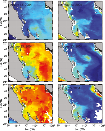
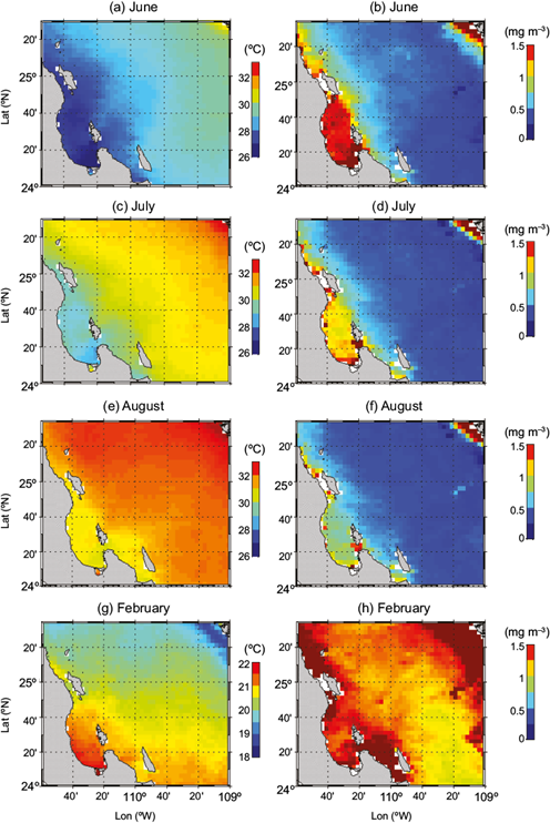
The fluorescence averaged in the top 50 m (Fig. 8) shows a maximum that coincides in position with the SST minimum (Fig. 4b); that is, it is located in the center of the cyclonic circulation. The coolness and chlorophyll (CHL) richness of the bay’s surface water (relative to the nearby waters of the Gulf) was apparent in the MODIS satellite images collected throughout the summer of 2004. Figure 9 shows examples of SST and CHL images for the weeks centered on May 13, June 23 and July 25. To prove that this is a recurrent summer feature of Bahía de La Paz, the weekly-mean SST and CHL MODIS time series of images comprising the bay and surrounding waters was harmonically-analyzed as described in section 2. Then the mean, the annual and the semiannual harmonics were used to construct the seasonal evolution of SST and CHL, part of which is shown in Figure 10, where the left panels show SST and the right panels show CHL, for the months of June, July, August and February.

Fig. 8 Fluorescence (relative units) averaged over the top 50 m of the water column during cruise NAME-II.
While the SST of the GC and the bay increases from June to August (Fig. 10a, c, e), the SST of Bahía de La Paz remains cooler than the surrounding southern GC. Moreover, Figure 10a, c shows an SST relative minimum nucleus inside the bay close to the center of the cyclonic circulation described above. The corresponding distributions of surface CHL for June, July and August (Fig. 10b, d, f) show that although the CHL decreased as the warm seas advanced, throughout the summer the bay maintained higher values of CHL than the adjacent GC. Furthermore, a relative maximum of CHL is found during these months approximately at the center of the cyclonic circulation described above. A contrasting situation is found in February (Fig. 10g, h): the SST inside the bay is slightly warmer than the surroundings, and the CHL is high everywhere in the southern GC, including the bay. Figure 10 also shows that the cool and CHL-rich summer conditions are not constrained to Bahía de La Paz, but are present in a narrow coastal band adjacent to the peninsula, north and south of the bay.
4. Discussion
During the observation period, there were two possible forcing mechanisms for the dynamics inside the bay: (i) the circulation outside the bay and (ii) the curl of the local wind stress. Of course, both mechanisms could act at the same time.
4.1 The outside currents
The hypothesis that the circulation in the GC could force a cyclonic circulation inside the bay was pointed out by Sánchez-Velasco et al. (2006), who supported this idea on the results of previous theoretical and numerical work on the annual circulation in the GC (Beier, 1997; Ripa, 1997). The proposed mechanism is that during the warm period a seasonal internal coastal trapped wave (trapped within ~70 km of the coast) runs cyclonically the whole periphery of the Gulf, and it could force the circulation in a deep basin with a wide entrance, like Bahía de La Paz. Evidence for forcing from outside are the surface distributions of salinity presented here (Fig. 4b) and by Monreal-Gómez et al. (2001), the distribution of fish larvae assemblages of Sánchez-Velasco et al. (2006) and the distribution of zooplankton biomass reported in Durán-Campos et al. (2015).
However, the circulation over the Southern GC during the NAME-II campaign was dominated by a train of cyclonic and anticyclonic eddies with diameters ~70 km (Zamudio et al., 2008; Lavín et al., 2013, 2014). In particular, during August 2004, at northeast of Bahía de La Paz bay a cyclonic eddy occupied much of the Farallón Basin and showed mean swirl speed of ~0.30 m s-1 and a mean core radius of 33 km (Lavín et al., 2013). The horizontal scale of the Gulf of California eddies is one order of magnitude larger than that of Bahía de la Paz, therefore in principle they are capable of forcing the circulation inside the bay. If the circulation inside the bay was forced by the Gulf of California eddies, then either sense of rotation could be induced, since they tend to occur with alternate vorticity (Pegau et al., 2002; Zamudio et al., 2008; Lavín et al., 2013, 2014). This would explain the observations of anticyclonic circulation inside the bay by Salinas-González et al. (2003) and could in part also explain the cyclonic circulation described in this work. Durán-Campos et al. (2015) suggested that the origin of the cyclonic eddy could be associated with the shape of the basin, like the interchange of the currents entering to the bay by the north mouth area and the bathymetric effect. No doubt there is a considerable interaction between the bay and the GC, but we consider that more observational and modeling work is necessary to establish this causal relationship for the bay’s circulation.
4.2 The wind stress curl
The upward displacement of the higher isothermals, DO and fluorescence isolines (Fig. 5), suggests that Ekman pumping induced by wind stress curl could partially contributed to the forcing mechanism of the cyclonic circulation. The wind stress observed in the bay during the August 2004 NAME-II cruise (not shown) was mainly from the south in the southern sector of the bay but rotated westward in the north basin; in principle this positive vorticity could be transferred to the basin. A wind pattern with positive vorticity was also observed in the June 1998 cruise of Monreal-Gómez et al. (2001). Despite this agreement on the sign of the wind stress curl in the two cruises, its effect on the circulation should be estimated with caution, since those measurements took place over only a couple of days, and the winds in Bahía de La Paz are notoriously variable, the breeze system is important (Turrent and Zaitsev, 2014; Cervantes-Duarte et al., 2021). It would be necessary to show that the correct wind stress curl was maintained for a sufficient length of time to generate the upward Ekman pumping, and that the magnitude of the wind stress curl at the appropriate time scale could produce a reasonable (i.e., as observed) displacement of the pycnocline.
The wind stress curl could cause an Ekman pumping, provided that the time scales involved are longer than f-1 (~4.6 days in Bahía de La Paz, ~24.5º N). If a positive wind stress curl is present during the summer as a seasonal forcing, it could explain the seasonal behavior of SST and CHL of the bay described above, by virtue of Ekman pumping decreasing the surface temperature and increasing the nutrients and therefore promoting the increase of phytoplankton (Coria-Monter et al., 2014; Herrera-Cervantes, 2019; Sánchez-Mejía et al., 2020). It would also contribute partially to the cyclonic circulation via isopycnal uplift.
The seasonal component of the wind and the wind stress curl in the southern Gulf of California, constructed the same way as the SST and CHL seasonal cycle (Fig. 10), are shown in Figure 11. During the summer period (June, July and August, Fig. 11a-c), the wind blows equatorward on the western side of the peninsula, parallel to the mountain ridge (Fig. 1b) (Castro and Martínez, 2010). However, the wind turns counterclockwise toward the GC over the peninsula and especially when it passes beyond its tip; inside the GC, from May to July it progressively blows to the northeast and then to the north (Bordoni et al., 2004; Lavín et al., 2009, 2014; Herrera-Cervantes et al., 2017). During February the wind blows from the northwest both in the Pacific and in the GC, and the wind stress curl was negative (positive) at east (west) side of the peninsula (Fig. 11d).

Fig. 11 Seasonal CCMP wind velocity (arrows, m s-1), and wind stress curl (color, 107 N m-3), during: (a) June, (b) July, (c) August, and (d) February.
The wind distribution causes the peninsula to be surrounded from June to August by a band of positive wind stress curl (Fig. 11a-c). The band on the Pacific side is caused by the lateral wind shear due to the presence of land, while the band that covers from the maximum curl south of the tip of the peninsula and along and off the gulf side of the peninsula is caused by the wind backing (i.e., turning counterclockwise). Bahía de La Paz is located within the coastal band of positive curl inside the GC, and it may present a relative maximum because it is located at the end of a topography gap connecting the Pacific lower atmosphere with that of the GC (Fig. 1b). The wind turning cyclonically at around 24º N is a possible mechanism for transferring positive vorticity to the bay at the seasonal time-scale. Trasviña-Castro et al. (2003) proposed a similar mechanism to explain the upwelling filaments caused by the Santa Ana winds in the Pacific coasts of northern Baja California, in a similar fashion as the generation of eddies in the Gulf of Tehuantepec by the Norte winds (see Willett et al., 2006 and references therein), but their time scales are a few days at most. The wind stress curl values seen in Figure 11a-c are very high (O[10-7 N m-3]), only comparable with those found in the Gulf of Tehuantepec (Chelton et al., 2004).
The upward Ekman pumping around the coasts of the peninsula caused by the cyclonic wind stress curl described above is additional to the upwelling generated by offshore Ekman transport caused by the along-shore winds in the presence of the solid coastal boundary. The latter depends only on the component of the wind stress parallel to the coast, while the former depends on the curl strength rather than on the wind stress intensity (Bakun and Nelson, 1991; Castro and Martínez, 2010). Both mechanisms are at work on both sides of the peninsula during summer (Fig. 11a-c), while in winter (Fig. 11d) only coastal upwelling is at work, off the Pacific side of the peninsula and off the mainland side of the GC. The across-gulf tilt of the isotherms noted by Lavín et al. (2009) in the southern GC during June 2004 may have been caused by a wind stress curl similar to that shown in Figure 10a, b, which is seen to change sign across the gulf’s axis.
To synthesize the seasonal behavior of wind stress curl, SST and CHL in Bahía de La Paz we space-averaged over the bay the respective weekly time series for the period 2003-2007; these weekly space-averaged time series are shown in Figure 12, together with their seasonal fits. The parameters of the seasonal fits are listed in Table II. It is noteworthy that the semiannual component is very important; in the case of the wind stress curl and CHL it is as important as the annual one.

Fig. 12 Time series of the average inside Bahía de La Paz of the CCMP wind stress curl (upper panel), MODIS SST (middle panel), and MODIS CHL (lower panel).
Table II Parameters of the seasonal fitting.
| Temporal mean | Annual amplitude | Annual phase | Semiannual amplitude | Semiannual phase | Explained variance | |
| SST | 25.3 ± 0.06 | 4.62 ± 0.08 | 15 August ±1 day | 1.10 ± 0.08 | 15 September ± 2 days | 94% |
| Curl | 0.53 ± .02 | 0.89 ± 0.03 | 30 June ± 1 day | 0.41 ± 0.03 | 2 October ± 2 days | 29% |
| CHL | 0.82 ± 0.03 | 0.40 ± 0.05 | 27 February ± 7 days | 0.31 ± 0.05 | 20 June ± 4 days | 31% |
The seasonal fit to the wind stress curl (Fig. 12a), which explained 30% of total variance, shows important mean positive values from May to August. Superimposed on the seasonal signal there are strong oscillations of the wind stress curl in a period of days (hence the low explained variance), but from May to August of each sampled year the seasonal signal dominated the variance in summer. Although the seasonal fit shows anticyclonic values during winter, the mesoscale variability and shorter time scale cause wide oscillation of the curl, from positive to negative values; these oscillations dominate the variance in winter. Superimposed to the seasonal fitting, there is strong non-seasonal variability in the wind stress curl which could increase the transfer of positive vorticity to the bay, for example during February-March 2006; or decrease the transfer of positive vorticity as in July-August 2003.
The SST and its seasonal fit are shown in Figure 12b. From May to August, when the wind stress curl is positive, the SST increases in Bahía the La Paz, just like in the entire GC, but as proved above the SST is cooler than in the Gulf, so that it lags its seasonal summer surface heating (Fig. 10). This lag can be related with the transfer of positive vorticity to the bay by the wind stress curl and the associated upward Ekman pumping of cool water. The bay-averaged CHL values and its seasonal fit are shown in Figure 12c. The seasonal variability shows high values of CHL from May to August, which correlates with positive wind stress curl. Note that the plumes of cool, chlorophyll-rich water apparently coming out of Bahía de La Paz seen in Figure 9 do not appear on Figure 10; this indicates that they are mesoscale structures with high variability.
Thus, during summer in Bahía de La Paz, the wind stress curl Ekman pumping brings cool, nutrient-rich subsurface water to the surface, causing chlorophyll enrichment of the upper layers (with maximum at the thermocline). This implies an input of sub-thermocline water into the bay, which by conservation has to be exported in the surface layers; this must be an important feature of the bay-gulf interaction. This could be the explanation of the cool, chlorophyll-rich plumes seen exiting Bahía de La Paz in Figure 9.
5. Conclusions
The first direct current observations (LADCP and surface drifters) in Bahía de la Paz concur with previous reports of cyclonic circulation in the northern sector of the bay. However, it was found that the centrifugal force cannot be neglected. This caused the cyclonic flow to be subgeostrophic; actual speeds (0.20-0.25 m s-1) were ~25-40% lower than those estimated from geostrophic balance (0.25-0.35 m s-1).
The observed hydrographic structure and the analysis of satellite data (wind velocity, SST and CHL), suggest that a partial mechanism on the contribution of the summer (June-August) cyclonic circulation, could be originated by Ekman pumping due to a strong positive wind stress curl. The process raises the thermocline/pycnocline closer to the surface than in the surrounding waters of the Gulf, causing the relative cooling and chlorophyll enrichment of the upper layers of the bay.

