


 nueva página del texto (beta)
 Inglés (pdf)
 Artículo en XML
 Referencias del artículo
 Enviar artículo por email
 Citado por SciELO
  Similares en
SciELO
Similares en
SciELO 
 Permalink
1. Introduction
Mexico’s geography entails a diversity of climates, which gives an agricultural potential for the yield of a vast range of crops. However, there is a lack of studies suggesting the best suitable crops in Mexico for different environments. Regularly, the choice of a crop in the country relies on the market, governmental subsidies and the farmer’s own interests.
Agriculture is the main economic activity in the state of Nayarit, using 602 407 ha (22% of the total state’s area), whereof 110 895 ha are irrigated and 491 512 ha are for non-irrigated farming (INEGI, 2011). There are three crop seasons: fall-winter (from October to January), encompassing over 39.1% of the farmland; spring-summer (from March to August), covering over 10.7%, and perennial (from January to December), involving 50.2% (SIAP, 2021). The irrigated and non-irrigated surface areas during the fall-winter season are 42.3 and 57.7%; 18.9 and 81.1% during spring-summer, and 11.2 to 88.8% for perennials (SIAP, 2021). The irrigated and non-irrigated surface areas during the fall-winter season are 41.6 and 58.4% of the total farmland; 16.9 and 83.1% during spring-summer, and 11.5 to 88.5% for perennials (SIAP, 2020). Main crops per cultivated surface area are: sorghum, corn, beans (Phaseolus vulgaris L.), sugar cane (Saccharum officinarum L.), and mango (Mangifera indica L.) (Gobierno del Estado de Nayarit-INEGI, 2017).
During 1995-2006, the state’s total production was less than 60 000 000 t per year and it has been decreasing since 1998. Despite the widest spread of agriculture in 2005 (a little more than 380 000 ha), the total crop yields were some of the lowest ever (20 000 000 t) (Zamudio and Méndez, 2011). The total crop surface during the 2016-2017 farming year was 61 213.62 ha and yielded 1 365 619.16 t per year, with an economic value of MXN 2 739 139 310 (Conagua, 2018). Such an agricultural productivity is low, despite the increase of agricultural surface in 2019 to 182 105.71 ha that yielded earnings of MXN 5 065 591 410 (SIAP, 2019).
This situation has a negative impact on the state’s economy. According to the state’s GDP (Gobierno del estado de Nayarit-SAGARPA, 2010), Nayarit has a low 11% contribution of the primary sector (23% secondary, and 66% tertiary), due to economic transformations that took place during the decade of 2010, when contributions of the primary sector began to decline (50%). At the national level, Nayarit contributed in 2018 with 0.7% of the GDP: 1.3, 0.4 and 0.8% of the primary, secondary and tertiary sectors, respectively (IIEG-Gobierno del Estado de Jalisco, 2020).
In the state of Nayarit, agriculture has two production systems: technology-based (with irrigation infrastructure, acceptable yields and sufficient profit margins), and dryland farming (with non-irrigated agriculture and low productivity), both co-existing in the same territory (included the only irrigation district within the state, DR-043) and even used in the same crops. DR-043 has an extension of 51 329 ha, whereof 29 864.8 ha were irrigated (99.3% using surface water and 0.7% with groundwater) during the 2018-2019 farm season (CONAGUA, 2021). Farmers in DR-043 have access to credits and technical assistance, allowing the use of agricultural technology for a better commercial performance.
Crop zoning encompasses a study aiming to limit areas for the adequate growing of one or more species of plants; therefore, ensuring good crop yields. Agroclimatic studies assess the climate with respect to the needs of a crop, whereas an agroecological study also takes into account limiting soil factors such as texture and depth, as well as the type of technology used for production.
Climate is key in agriculture (Villa et al., 2001) and allows for the correct management of crops (White et al., 2001). Environmental temperature is one of the most important climatic and meteorological factors for plant growth, determining spatial distribution of natural vegetation and the suitability of crops (Lozada and Sentelhes, 2008). Temperature directly influences the physiological processes of the plant such as respiration, mineral absorption, photosynthesis, growth, flowering and water balance (Aguilar et al., 2010).
Cold and heat intensity and duration affect metabolic activity, plant growth and viability, thus, limiting the geographic distribution of crops. Temperature and precipitation are the most relevant indicators, since the former closely determines biological processes, while the latter determines vegetation cover and crop productivity (Allen et al., 1989). It is important, however, to include solar radiation since it sets the conditions of insolation, photoperiod, photosynthesis and the real and potential evapotranspiration (Velasco and Pimentel, 2010). The long and slow process of adaptation of crop plants to natural environments in the sake of better yields, turn them more susceptible to climate than wild plant communities. The decline in resistance counteracts the gain in productivity, with serious impact on agriculture.
The aim of this study was to undertake the agroclimatic zoning of the state of Nayarit, based on Papadakis’ climate classification system (PCCS) (Papadakis, 1970), in order to determine the most convenient crops to obtain highest yields. The zoning system used for this purpose, which is also used in Spain (Lozano et al., 2000), is probably the best known and most applied worldwide (Velasco and Pimentel, 2010).
2. Materials and methods
2.1 Study area
Nayarit (23º 05’-20º 36’ N; 103º 43’-105º 46’ W) is a state in central Mexico with an extension of 27 621 km2, limiting to the north with Sinaloa and Durango, to the east with Durango, Zacatecas and Jalisco, to the south with Jalisco and the Pacific Ocean, and to the west with the Pacific Ocean and Sinaloa. Twenty-five weather stations (WS) distributed across Nayarit and bordering states (whose geographical locations are listed in Table I) were selected for this study.
Table I Geographical location and climate conditions of the weather stations (WS) in Nayarit and surrounding states (1951-2010).
| Weather stations | Code | Latitude | Longitude | Altitude (masl) | ATmean (˚C) | ATmax (˚C) | ATmin (˚C) | APmean (mm) | ATE (mm) | |
| Durango | Las Bayas | 10040 | 23º 30’ 16” | 104º 49’ 28” | 2643 | 11.1 | 20.2 | 2.1 | 1040.1 | NA |
| Jalisco | Bolaños | 14023 | 21º 49’ 30” | 103º 47’ 00” | 963 | 24.4 | 33.6 | 15.2 | 593.3 | 1902.3 |
| Hostotipaquillo | 14068 | 21º 03’ 52” | 104º 03’ 05” | 1300 | 21.7 | 30.1 | 13.2 | 838.5 | 1958.7 | |
| San Gregorio | 14125 | 20º 37’ 15” | 104º 34’ 05” | 1640 | 15.4 | 23.9 | 6.9 | 1305.1 | 1365.6 | |
| Tenzompa | 14306 | 22º 22’ 34” | 103º 55’ 29” | 1770 | 16.8 | 26.2 | 7.3 | 698.7 | 2124.4 | |
| Nayarit | Acaponeta | 18001 | 22º 29’ 24” | 105º 21’ 15” | 24 | 25.9 | 33.3 | 18.5 | 1325 | 1896.7 |
| Amatlán de las Cañas | 18003 | 20º 48’ 00” | 104º 24’ 00” | 798 | 24.9 | 34.1 | 15.6 | 800.3 | NA | |
| Capomal | 18004 | 21º 50’2 2” | 105º 07’ 16” | 35 | 26.1 | 33.3 | 18.9 | 1529 | 1821.1 | |
| Despeñadero | 18008 | 21º 50’ 29” | 104º 43’ 21” | 315 | 26.7 | 33.7 | 19.8 | 846.5 | 2409.9 | |
| El Carrizal | 00018045 E | 21º 49’ 38” | 104º 34’ 30” | 632 | 28.3 | 35.2 | 21.4 | 1155 | 2086.5 | |
| El Naranjo | 18085 | 22º 02’ 03” | 104º 51’ 43” | 239 | 27.2 | 34.3 | 20.1 | 1378.6 | 1799.6 | |
| Huaynamota | 18014 | 21º 55’ 11” | 104º 30’ 49” | 670 | 25.2 | 33.9 | 16.4 | 853.5 | NA | |
| Jumatan (CFE) | 18019 | 21º39’00” | 105º 02’ 00” | 359 | 23.9 | 30.4 | 17.5 | 1443.7 | 1443.9 | |
| La Yesca | 18020 | 21º 19’ 28” | 104º 00’ 45” | 1357 | 27.5 | 36.2 | 18.8 | 743 | 2437.1 | |
| Las Gaviotas | 18021 | 20º 53’ 23” | 105º 08’ 12” | 56 | 26.1 | 33.4 | 18.9 | 1577.6 | 1699 | |
| Pajaritos | 18068 | 22º 22’ 40” | 105º 15’ 15” | 76 | 25.2 | 32.6 | 17.8 | 1349.4 | 1898.2 | |
| Paso de Arocha | 18025 | 21º 16’ 31” | 105º 04’ 52” | 84 | 25 | 31.3 | 18.7 | 1685.4 | 1558.8 | |
| Rosamorada | 18028 | 22º 07’ 20” | 105º 12’ 14” | 30 | 25.7 | 33.2 | 18.2 | 1361.1 | 1707.4 | |
| San José Valle | 18030 | 20º 44’ 38” | 105º 13’ 46” | 20 | 27.4 | 33.8 | 21.1 | 1071.3 | 1810 | |
| San Juan Peyotán | 18031 | 22º 21’ 40” | 104º 25’ 54” | 639 | 25.1 | 35 | 15.1 | 848.2 | 1963.3 | |
| San Marcos | 18080 | 20º 57’ 25” | 105º 21’ 12” | 7 | 25.9 | 33.3 | 18.6 | 1051.3 | ||
| Tecuala | 18036 | 22º 24’ 20” | 105º 27’ 30” | 10 | 25 | 32.4 | 17.7 | 993.8 | 1609.6 | |
| Tepic | 18038 | 21º 30’ 00” | 104º 53’ 00” | 935 | 20.3 | 27.5 | 13.1 | 1239.9 | 1807.5 | |
| Zacualpan | 18043 | 21º 15’ 00” | 105º 10’ 00” | 29 | 25 | 30.8 | 19.1 | 1375.7 | NA | |
| Sinaloa | Ototitán | 25186 | 23º 00’ 50” | 105º 40’ 00” | 93 | 26.3 | 35 | 17.5 | 913.7 | NA |
ATE: annual total evaporation; APmean: annual average precipitation; ATmean: annual average temperature; ATmax: annual maximum temperature; ATmin: annual minimum temperature; NA: non-available.
Source: SMN, 2019.
The types of climate in Nayarit and the percentages of the state area they encompass are: hot humid with heavy rainfall in summer (Am), 0.56%; hot sub-humid with summer rainfall (A[w]), 60.63%; warm sub-humid with summer rainfall (ACw), 30.96%; temperate sub-humid with summer rainfall (C[w]), 6.15%, and semi-arid very hot and hot (BS1[h’]), 1.7% (INEGI, 2018) (Fig. 1). The average annual temperature is 25 ºC, the minimum average temperature is 10 ºC in January, whereas the maximum average temperature is about 35 ºC in May and June. The raining season is in summer (May through September), averaging an annual precipitation of 1100 mm (García, 2004) (see Table I for greater detail).

Nayarit has a wide range of soil types (Table II): Acrisol, Andosol, Arenosol, Cambisol, Fluvisol, Gleysol, Leptosol, Luvisol, Nitisol, Phaeozem, Regosol, Solonchak, Umbrisol and Vertisol (INEGI, 2018). The type of land is distributed within the state as follows: agriculture (15.9 %), grassland (14.6 %), livestock (61.2 %), woodland (4.9 %), and non-productive (3.4 %) (Bojórquez et al., 2006). Nayarit is divided into four hydrological regions: Presidio San Pedro, Lerma-Santiago, Huicicila and Ameca. The main rivers across the state are Acaponeta, San Pedro, Santiago, Huicicila and Ameca. Freshwater bodies and salty ponds are the Aguamilpa, San Rafael and Amado Nervo dams, and the Agua Brava lake.
Table II Soil types in the state of Nayarit, Mexico.
| Name/code | Characteristics | Surface (%) |
| Acrisol (AC) | Low-activity clay soil, acid and infertile for agriculture, common in rainy areas, red tone or light yellow with red spots, susceptible to erosion if logging and root removal. | 1.91 |
| Andosol (AN) | Andosols accommodate soils that develop in glass-rich volcanic ejecta under almost any climate. Andosols have a high potential for agricultural production, they are generally fertile soils. The strong phosphate fixation of Andosols (caused by active Al and Fe) is a problem. | 0.57 |
| Arenosol (AR) | Arenosols have high permeability and low water and nutrient storage capacity. Arenosols offer ease of cultivation, rooting and harvesting of root and tuber crops. | 0.78 |
| Cambisol (CM) | Cambisols combine soils with at least an incipient subsurface soil formation. Transformation of parent material is evident from structure formation and mostly brownish discoloration, increasing clay percentage, and/or carbonate removal. Cambisols make good agricultural land and are used intensively. | 21.46 |
| Fluvisol (FL) | Soils developed in fluvial, lacustrine and marine deposits, no groundwater and no high salt contents in the topsoil. Good natural fertility. | 1.90 |
| Gleysol (GL) | Gleysols comprise soils saturated with groundwater for long enough periods to develop reducing conditions resulting in gleyic properties. Redox processes are caused by ascending gases (CO2, CH4). | 0.11 |
| Leptosol (LP) | Leptosols comprise very thin soils over continuous rock and soils that are extremely rich in coarse fragments. Thin soils with various kinds of continuous rock or of unconsolidated materials with less than 20% (by volume) fine earth. | 15.49 |
| Luvisol (LV) | Luvisols have a higher clay content in the subsoil than in the topsoil, as a result of pedogenetic processes (especially clay migration) leading to an argic subsoil horizon. Luvisols have high-activity clays throughout the argic horizon and a high base saturation in the 50-100 cm depth. | 16.11 |
| Nitisol (NT) | Nitisols are deep, well-drained, red tropical soils with diffuse horizon boundaries and a subsurface horizon with at least 30 percent clay and moderate to strong. The deep and porous solum and the stable soil structure of Nitisols permit deep rooting and make them quite resistant to erosion. | 0.94 |
| Phaeozem (PH) | Phaeozems accommodate soils of relatively wet grassland and forest regions in moderately continental climates. Dark soils rich in organic matter. Phaeozems are porous, fertile soils and make excellent farmland. | 12.13 |
| Regosol (RG) | Regosols are very weakly developed mineral soils in unconsolidated materials. Not very thin, unconsolidated, generally fine-grained material. Regosols in desert areas have minimal agricultural significance. | 15.92 |
| Solonchak (SC) | Solonchaks have a high concentration of soluble salts at some time in the year. Arid and semi-arid regions, notably in areas where ascending groundwater reaches the upper soil or where some surface water is present, with vegetation of grasses and/or halophytic herbs, and in inadequately managed irrigation areas. | 5.38 |
| Umbrisol (UM) | Umbrisols have a significant accumulation of organic matter in the mineral surface soil and a low base saturation somewhere within the first meter (in most cases in the mineral surface soil). Soils with dark topsoil. Weathering material of siliceous rock or of strongly leached basic rock. | 2.59 |
| Vertisol (VM) | Vertisols are heavy clay soils with a high proportion of swelling clays. These soils form deep wide cracks from the surface downward when they dry out, which happens in most years. Sediments that contain swelling clays, or swelling clays produced by neoformation from rock weathering. | 1.21 |
| Others | Different types of soils with minimal non-mappable areas. | 3.5 |
Source: INEGI, 2018; IUSS Working Group WRB, 2015.
2.2 Methodology
The agroclimatic zoning was based on PCCS (Papadakis, 1970), which relies on climate variables such as average, maximum and minimum temperatures, annual and monthly rainfall, and potential evapotranspiration. The information from the 25 WS was gathered from data records (1951 to 2010) provided by Mexico’s National Weather Service (SMN, 2019).
PCCS classifies geographic regions into 10 climatic groups, according to three dimensions: winter and summer types, and humidity patterns. These groups are cold land, desert, Mediterranean, Pampean and tropical (nine subdivisions each); polar alpine and subtropical (five subdivisions each); marine and steppe (eight subdivisions each); and continental humid (three subdivisions). PCCS includes a list of 186 special diagnostics used to define each group’s subdivisions.
PCCS underlines the concept of monthly climate based on thermic and hydric characteristics, identifying 29 monthly thermic climates according to the average temperatures and extremes (maximum and minimum); and seven monthly hydric climates, composed by monthly precipitation plus the volume of water stored in soil due to previous rainfalls.
Arid climate (a) is defined when a set of climate variables entails less than 25% of the potential evapotranspiration; dry (s), between 25 to 50%; dry hydric intermediate (i), 50 to 75%; humid hydric intermediate (y), 75 to 100%; post-humid (p), more than 100%; humid (h), if rainfall denotes more than 100%; hyper-humid (w), when precipitation plus the soil moisture stored from previous rainfalls account for more than 200% of the potential evapotranspiration (Papadakis, 1970). PCCS computes evapotranspiration based on mid-day saturation deficit. The three PCCS dimensions were calculated using the climatic information from each WS.
2.2.1 Calculation of winter climate types
Data used correspond to the coldest month based on the average of absolute minimum temperatures (T pb ), the average of minimum temperatures (T min ), and the average of maximum temperatures (T max ). T pb was calculated as follows:
From these values, the types of winter climate were determined for each WS according to criteria shown in Table III.
Table III Winter and summer climate types in Mexico according to Papadakis (1970).
| Winter type*/ characteristics | Tpb | Tmín | Tmáx | Summer type/ Characteristics | FFPmín | FFPavail | TMax | Tx6 | Tx4 |
| (ºC) | (months) | (ºC) | |||||||
| Equatorial (Ec) | >18 | Cotton (G) | >4.5 | >33.5 | >25 | ||||
| Tropical (Tp) | > 7 | 13-18 | Cotton (g) | >4.5 | <33.5 | >25 | |||
| Tropical (tP) | > 7 | 8-13 | >21 | Coffee (c)** | 12 | <33.5 | >21 | ||
| Tropical (tp) | > 7 | 8-13 | <21 | Rice (O) | >3.5 | >25.0 | >21 | ||
| Citrus (Ct) | -2.5 a 7 | >8 | >21 | Maize (M) | >4.5 | >21 | |||
| Citrus (Ci) | -2.5 a 7 | >8 <8 | 10-21 >21 | Triguera cálida (T) | >4.5 | >17 | |||
| Oat (Av) | -10 a -2.5 | >4 | >10 | Wheat (t) | 2.5-4.5 | >17 | |||
| Oat (av) | -10 a -2.5 | >4 <4 | 5-10 >10 | Andine-alpine (A) | >1 | >10 | |||
| Triticum (Tv) | -29 a -10 | > 5 | |||||||
| Triticum (Ti) | -29 a -10 | 0 y 5 | |||||||
*Based on coldest month of the year; **all months with Tmax < 33.5 and Tmín < 20 ºC.
Tpb: average of absolute minimum temperatures; Tmin: average of minimum temperatures; Tmax: average of maximum temperatures; FFPmin: minimum frost-free period; FFPavail: available FFP; Tmax: highest temperature registered for the month with the highest average temperature; T × 6: average temperature of the six hottest months of the year according to Tmean; T × 4: average temperature of the four hottest months based on Tmean.
Source: authors’ self-preparation based on Papadakis (1970) information.
2.2.2 Calculation of summer climate types
This process included the frost-free period (FFP) and T max from different months. FFP was calculated using T pb in two forms: minimum FFP (FFP min ), where monthly T pb > 7.0 ºC; and available FFP (FFP avail ), when monthly T pb > 2.0 ºC. Hence, it was necessary to know the T pb of every month of the year.
T max was used in four ways: (1) T max of the month whose average temperature (T mean ) was the highest along the year; (2) average temperature of the six hottest months of the year (T × 6), according to T mean ; (3) average temperature of the four hottest months (T × 4) based on T mean , and (4) average of maximum temperatures for all months in a year. Then, the types of summer climate could be determined for each WS according to criteria shown in Table III.
2.2.3 Humidity pattern
The humidity pattern refers to the natural availability of water for plants, based on three indices calculated from the water balance in soil (Thornwaite, 1948) to store up to 100 mm of water: annual humidity, monthly humidity and lixiviated rainfall. Monthly hydric characteristics were calculated using precipitation data, monthly potential evapotranspiration (PET) and the amount of water stored in the soil from previous rainfalls. Water balance facilitated the estimation of PET (Elías et al., 2001):
where PET is the potential evapotranspiration (mm); e a the vapor pressure to saturation (mbar) computed with the highest average temperature; e mi-2 the vapor pressure to saturation (mbar) computed with the lowest average temperature minus two Celsius degrees. Both vapor pressure variables were calculated as follows:
Water balance was performed using Excel software. The months of the year were listed on the spreadsheet followed by data in columns about precipitation (P), PET and P-PET. This latter column allowed the identification of the month in which water balance began, i.e., setting the first month when P > PET, since a positive value indicates water excess.
From that month on, the positive value filled in the column named “exceeding” in the worksheet, adding the P-PET value of the following month as long as it was also positive. The process was repeated until a negative value was obtained, indicating the end of water excess, and thus, a zero value was registered in the column. PCCS deems the water storage capacity of the soil to 100 mm, the highest value possible, although the sum could be even higher.
The positive value of the excess column was subtracted from the column named “water used” (water amount to meet the PET requirements), repeating the process every month until depletion or negative values were obtained. Water balance allowed for the calculation of monthly and annual humidity indices, and the lixiviated rainfall as well, for the wet season.
2.2.3.1 Annual humidity index (HIA )
The HI A was calculated according to the following equation:
where P is precipitation (mm) and PET evapotranspiration (mm), both annually. HI A determined the hydric pattern of the CS.
2.2.3.2 Monthly humidity index (HI m )
The HI m allowed differentiating wet months (H; with HI m > 1.0) from intermediate (I; 0.5 < HI m < 1.0) and dry (S; with HI m < 0.5). This index was estimated using water consumption data:
where P m is the monthly precipitation (mm), water used m is water used in the month (mm) and PET m is the monthly evapotranspiration (mm). In cases where there was no water consumption, HI m was calculated as follows:
2.2.3.3 Lixiviated rainfall (L n )
L n is composed by the sum of differences of P-PET from the wet months, expressed as mm (Eq. [8]) and in percentage (Eq. [9])
where P is precipitation (mm), PET potential evapotranspiration (mm), and the wet months were those whose P-PET value was positive, confirmed by HI m . The humidity pattern was determined for all WS using HI A and HI m Ln data calculated from a list of 186 PCCS special diagnostics (Table IV).
Table IV Climate patterns of Mexico according to Papadakis (1970).
| Humidity pattern | Characteristics |
| Humid | HIA > 1, Ln (%) > 0.20 of PET |
| HU: all months wet | |
| Hu: at least one month dry | |
| Monsoon | Humid monsoon (MO): Ln (%) > 0.20 of PET and HIA > 0.88 |
| Dry monsoon (Mo): Ln (%) < 0.20 of PET; 0.44 < HIA < 0.88 | |
| Semiarid monsoon (mo): HIA < 0.44 | |
| Desert | Desert: all months with T > 15 ºC are dry; HIA< 0.22 |
| Absolut desert (da): HIm < 0.25, for all months with Tmax> 15 ºC, HIA < 0,09 | |
| Mediterranean desert (de): not dry enough for da; winter rainfall greater than summer | |
| Monsoon desert (do): not dry enough for da; July-August less dry than April-May | |
| Isohigro desert (di): not da, nor de or do |
PET: potential evapotranspiration; HIA: annual humidity index; HIm: monthly humidity index; Ln: lixiviated rainfall; Tmax: average of maximum temperatures.
Special diagnostics: the complete list of 186 diagnostics is not included in this document. For more information refer to Papadakis (1970).
2.2.4 Agroclimatic zoning map
The software ArcMap v. 10.5 was used to make the agroclimatic zoning map based on the shape files of geographic metadata provided by the National Commission for the Knowledge and Use of Biodiversity (CONABIO, 2008) and the National Water Commission (CONAGUA, 2021), using the cross-sectional Mercator projection system, datum WGS 1984. For the calculation of climatic variables, the inverse-distance weighted (IDW) interpolation method was appropriate since they depend on the geographical location.
The map combines regions with similar climate, first dividing them into small units (cells) with similar climatological conditions. Then, the IDW computes each cell values through a weighted lineal combination from a set of sample points, which is a function of the inverse distance. Surface interpolation is a dependent variable of the geographical site (ESRI, 2016), which for this study was the climatic groups and subgroups of the PCCS.
3. Results and discussion
3.1 Determination of winter climate types
Temperature data from 1951 through 2010 of almost all CS records, identified January as the coldest month of the year, except in La Yesca (December), San Marcos and Zacualpan (both in February). The lowest T pb , T min and T max on that month were measured in Las Bayas (-6.6, -1.7 and 17.7 ºC) and Tenzompa (-3.9, 0.8 and 22.1 ºC) (Fig. 2); the highest, in El Carrizal (14.5, 17.7 and 32.4 ºC).
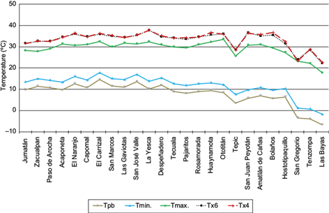
Fig. 2 Temperature records for coldest months (December-February) in participating climate stations (1951 to 2010).
CS were assigned to the following type of winter climates: 17 stations in tropical zone (Tp [hot], tP [warm]); five in the citric zone (Ct [tropical], Ci [typical]); and three in the oat zone (av) (Table V).
Table V Climatic groups of the study zone based on Papadaki’s Climate Classification System (PCCS) (1970).
| Weather station | Groupand subgroup | SD* | Climatic Group | Climatic Subgroup | Winter type | Summer ype | Humidity Pattern | Area (ha)** |
| Jumatán | 1.32 | 4, 63 | Tropical | Marine savanna tropical | Tp | g | Mo | 72 603.56 |
| Zacualpan | 1.32 | 4, 63 | Tropical | Marine savanna tropical | Tp | g | Mo | |
| Paso de Arocha | 1.37 | 4, 63, 95 | Tropical | Marine savanna tropical | Tp | g | MO | |
| Acaponeta | 1.42 | 64 | Tropical | Continental savanna tropical | Tp | G | Mo | 504 856.40 |
| El Naranjo | 1.42 | 64 | Tropical | Continental savanna tropical | Tp | G | Mo | |
| Capomal | 1.42 | 64 | Tropical | Continental savanna tropical | Tp | G | Mo | |
| El Carrizal | 1.42 | 64 | Tropical | Continental savanna tropical | Tp | G | Mo | |
| San Marcos | 1.42 | 64 | Tropical | Continental savanna tropical | Tp | G | Mo | |
| Las Gaviotas | 1.42 | 64 | Tropical | Continental savanna tropical | Tp | G | Mo | |
| San José Valle | 1.42 | 64 | Tropical | Continental savanna tropical | Tp | G | Mo | |
| Despeñadero | 1.533 | 35 | Tropical | Semiarid tropical | Tp | G | mo | 1010 722.42 |
| La Yesca | 1.534 | 0 | Tropical | Semiarid tropical | Tp | G | mo | |
| Tecuala | 1.915 | 36 | Tropical | Cool-winter tropical | tP | G | Mo | 893 481.53 |
| Pajaritos | 1.915 | 36 | Tropical | Cool-winter tropical | tP | G | Mo | |
| Rosamorada | 1.915 | 36 | Tropical | Cool-winter tropical | tP | G | Mo | |
| Ototitán | 1.916 | 35 | Tropical | Cool-winter tropical | tP | G | mo | |
| Huaynamota | 1.917 | 33 | Tropical | Cool-winter tropical | tP | G | mo | |
| San Gregorio | 2.4 | 1 | Cold land | High cold land β | av | t | Hu | |
| Tenzompa | 2.44 | 1 | Cold land | High cold land β | av | t | mo | |
| Las Bayas | 2.6 | 1 | Cold land | High Andine β | av | a | Mo | |
| Tepic | 4.24 | 0 | Subtropical | Continental subtropical | Ci | g | Mo | 191 950.46 |
| Bolaños | 4.31 | 32 | Subtropical | Continental semitropical | Ct | G | mo | 88 485.63 |
| San Juan Peyotán | 4.321 | 33 | Subtropical | Continental semitropical | Ct | G | mo | |
| Amatlán Cañas | 4.321 | 35 | Subtropical | Continental semitropical | Ct | G | mo | |
| Hostotipaquillo | 4.4 | 106 | Subtropical | Marine semitropical β | Ct | g | mo |
Winter types: av: Avena (oats) zone; Ct: citrus zone (average daily maximum of the coldest month > 21 ºC); Ci: citrus zone (average daily maximum of the coldest month between 10-21 ºC), Tp: tropical zone (average of the lowest coldest month > 7 ºC, average daily minimum of the coldest month between 13-18 ºC); tP: tropical zone (as for Tp, but average daily minimum of the coldest month between 8-13 ºC, average daily maximum of the coldest month >21 ºC).
Spring types: a: Andine-Alpine zone; G: Gossypium (cotton) zone (average daily maximum of the warmest month > 33.5 ºC); gϷ: Gossypium (cotton) zone (as for G, but average daily maximum of the warmest month < 33.5 ºC); t: Triticum (wheat) zone.
Humidity regimen: MO: rainy monsoon; Mo: dry monsoon; mo: semiarid monsoon; Hu: humid.
*Special diagnostics: the complete list of 186 diagnostics is not included in this document (or more information refer to Papadakis, 1970); **climatic subgroups determined by PCCS, however WS located outside the state of Nayarit.
3.2 Determination of summer climate types
All of the CS recorded T pb > 2.0 ºC all year round (i.e., frost free), except for Amatlán de Cañas (11 months of FFP min ); Bolaños, Hostotipaquillo and San Juan Peyotán (nine months); Tepic (five months); San Gregorio and Tenzompa, (four months); and Las Bayas (none). Also, all WS recorded a 12-month FFP avail except Las Bayas, San Gregorio and Tenzompa, which registered FFP avail during one, six and seven months, respectively.
La Yesca (40.6 ºC) was the WS with the highest T max value, whereas Las Bayas (23.4 ºC) had the lowest; T × 6 of La Yesca was 37.6 ºC and for Las Bayas 22 ºC; T × 4 for the same WS was 37.6 and 22.55 ºC, respectively (Fig. 2). According to the data obtained, the number of CS assigned to types of summer climates were as follows: 23 to the cotton zone (17 to the hottest [G]; five to the mild hot or warm [g]); one to an alpine zone (a), and two to the wheat zone (t) (Table V).
3.3 Humidity pattern determination
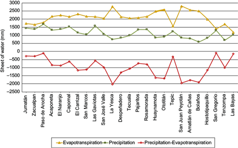
According to the humidity patterns, CS with extreme rainfall values were Paso de Arocha (1685.4 mm) and Bolaños (593.3 mm); extreme PET values were observed in San Juan Peyotán (2797.68 mm) and Las Bayas (1188.32 mm); in the rest of the CS, intermediate amounts were recorded (Fig. 3). However, all CS had higher PET values than P, which indicates an important water flow across the soil-plant-atmosphere system. As for the water balance, the highest PET value was recorded at La Yesca (-2028.16 mm). The WS with lowest P-PET values were San Gregorio (-89.2 mm) and Paso de Arocha (-106.59 mm).
The number of CS that exhibited a particular hydric pattern were: one humid (Hu) (HI A > 1 and L n > 20%) and 24 monsoon (14 dry monsoon [Mo; 0.44 < HIA < 0.88 and Ln < 20%]; 9 semi-arid monsoon [mo; HIA < 0.44]; and one rainy monsoon [MO; HIA>0.88]) (Table IV). CS were associated with three climate groups, according to the winter and summer types, hydric patterns and special diagnostics (Table V). Nevertheless, subtropical and tropical climatic groups are found only in Nayarit. The cold land group was registered in WS located in surrounding states (Table V).
3.4 Agroclimatic zoning and recommended crops
Figure 4 shows the agroclimatic zoning of the state of Nayarit, followed by the analysis based on the three climatic groups and the respective subgroups identified.

3.4.1.1 Cool-winter tropical subgroup
Non-irrigated winter potato (Solanum tuberosum L.) and rice (Oryza sativa L.) render high yields. Olives and grapes also grow well; however, since the summer is long and humid, they require fungicides and growth regulators for pest control and the use of irrigation during the dry season as well. Marginal progress is observed on winter cereals such as oat (Avena sativa L.), barley (Hordeum vulgare L.), rye (Secale cereale L.) and wheat (Triticum aestivum L.); and summer cereals such as rice, corn (Zea mays L.), temperate millet (Panicum miliaceum L.), pearl millet (Pennisetum cinereum Stapf & C.E. Hubbard) and sorghum (Sorghum bicolor [L.] Moench). All of them need irrigation, fertilizers and growth regulators, and require close attention to sowing dates: grains are hard to store when harvested during the wet season, whereas in the dry season, they could be damaged.
Therefore, it is recommended to sow at the beginning of the wet period, even though the harvest will take place under rainy weather. For instance, corn is sowed at the start the wet season, whereas sorghum and millet are sowed afterwards in order to be harvested and stored in the dry period. Non-irrigated rice is planted if the dry season is longer than five months, but the storage may turn difficult when it is harvested during rainfall. In all cases, there is a need of fertilizers, growth regulators and grain driers. Table VI shows recommended crops for Nayarit according to PCCS groups and subgroups identified.
Table VI Crops with improved yields, according to climate groups in Papadakis’ (1970) system.
| Climate group | Subgroup | Winter cereal | Summer cereal | Other crops | |||||||||||||||
| Oats | Rye | Barley | Wheat | Rice | Corn | Millet | Sorghum | Olives | Cotton | Banana | Sugarcane | Citric | Forage | Potato | Beetroot | Tea | Grapes | ||
| Tropical | Cool-winter tropical | - | - | - | - |

|
|
|
|
|
- | - |
|
|
- |
|
- | - |
|
| Continental savanna tropical | - | - | - | - |
|
|
|
|
- |
|
|
|
|
- | - | - | - | - | |
| Marine savanna tropical | - | - | - | - |
|
|
|
|
- |
|
|
|
|
- | - | - | - | - | |
| Semiarid tropical | - | - | - | - |
|
|
|
|
- |
|
|
|
|
|
- | - | - | - | |
| Subtropical | Marine semitropical |
|
|
|
|
|
|
- | - | - | - | - |
|
|
- |
|
- | - | - |
| Continental semitropical |
|
|
|
|
|
|
- |
|
|
|
|
|
|
|
|
|
- |
|
|
| Subtropical continental |
|
|
|
|
|
|
|
|
|
|
|
|
|
|
|
|
- |
|
|
| Cold land | High Andine | - | - | - | - | - |
|
- | - | - | - | - | - | - | - |
|
- | - | - |
| High cold land |
|
|
|
|
|
|
|
|
- | - | - |
|
- | - |
|
- | - | - | |
3.4.1.2 Continental tropical savanna subgroup
The continental savannah subgroup is excellent for irrigated banana and citric. Coconuts (Cocos nucifera L.) grow in high water-retention capacity soils; cotton has low yields and may develop sanitary problems; and forages may grow with low quality. This type of climate has the same features as the cool-winter tropical for winter and summer cereals described before. Sugar cane and forages grow with poor sugar content and nutrients, hence the need for growth regulators and nitrogen-based fertilizers, respectively.
3.4.1.3 Marine tropical savanna subgroup
Summer cereals are planted in regions with tropical marine savannah climate, using growth and respiratory regulators to control the effect of warm nighttime, as well as fertilizers to increase crop yields. Corn yields an optimal production if harvested during the dry season, and cotton, banana, sugar cane and citric require irrigation. This type of climate is too hot for coffee (Coffea spp.) and beet crops (i.e., very low yields). Forages produce low-protein levels.
3.4.1.4 Semiarid tropical subgroup
Semiarid tropical climate is good for irrigated summer cereals, and renders good yields if growth regulators and fertilizers are used and harvesting takes place during the dry season. Protein content in forage grains is usually low. Banana (with irrigation), sugar cane, and non-irrigated cotton and citric grow efficiently. According to Díaz-Padilla et al. (2012), Nayarit exhibits excellent agroclimatic conditions to increase the cropland for Persian lime (Citrus latifolia Tan.) production. These authors identified 418 000 ha with high potential productivity for this crop.
3.4.2.1 Marine semitropical subgroup
Winter cereals are produced properly by irrigation or in rainwater storing soils. Potato is an autumn or spring crop, whereas sugar cane corresponds to winter season. Summer cereals need no irrigation; however, rice grows better when is irrigated. On the other hand, millet and sorghum are more affected than corn due to warmer nights. This climate is humid, therefore, inadequate for cotton. Citrus may grow well without irrigation, whereas banana and sugar cane thrive in FFP regions. Fertilizers and growth regulators in winter and summer cereals increase crop yields.
3.4.2.2 Continental semitropical subgroup
Winter and summer cereals such as non-irrigated sorghum, irrigated corn and rice grow well in the absence of low temperatures. Warm nights in summer enhance crops growth. In some cases, accelerated growth affects sugar storage and nutrition of plants, hence, growth regulators and nitrogen-based fertilizers are needed to overcome the problem and still obtain good yields. The warmer nights of summer time foster the growth of all crops; therefore, the use of nitrogen-based fertilizers in addition to grow regulators is recommended to obtain better yields.
Other irrigated crops for this type of climate with FFP are cotton, alfalfa (Medicago sativa L.), banana and citric (favors orange’s color); sugar cane is recommended where winter presents few freezing events; olives and grapes grow well where one or more months are humid, but it is possible to face disease problems in plants and excessive root grow. Spring and autumn potato are good for short winters, and beet for winter.
3.4.2.3 Continental subtropical subgroup
In zones with continental subtropical climate, recommended crops are irrigated alfalfa, banana and citric (in FFP), winter cereals, beet and spring or autumn potato where winter cold gets mild. Fertilizers and growth regulators are necessary in order to render good yields, since summer nights tend to be warmer. Olives and grapes grow well without irrigation in zones where one or two months of summer are humid; however, only some types of summer cereals are appropriate.
3.4.3.1 High Andean subgroup
This climate is too cold for winter crops, such as sugar cane and potato (except wild potato [S. acaule Bitter]). As for winter cereals, only corn grows but with restrictions, due to low temperatures reached at night. Lowest temperatures recorded in this type of climate are also inconvenient for cotton, banana, coffee, citrus and tea.
Winter cereals may be planted in spring or autumn, but irrigation and fertilizer applications are necessary. For middle-term crops, such as sugar cane and potato, irrigation is compulsory, although it could be expensive for the farmer. This climate is rather cold-fresh for summer cereals, but corn may grow with the limitations imposed by cold nights. It is not recommended for cotton, banana, coffee, citrus and tea.
3.5 Agroclimatic zoning of PCCS and its relation to the climatic conditions of Nayarit
Based on García’s classification system (García, 2004), the main climate types distributed across the state’s surface are hot subhumid with summer rainfall (60.63%), and warm subhumid with summer rainfall (30.96%) (INEGI, 2018). Comparing this information with our study results, we found similar characteristics matching the tropical and subtropical climatic groups of the PCCS. respectively, where most of the WS are located (Fig. 1).
The largest surface area when zoning with the PCCS corresponded to semiarid tropical climate (1 010 722.42 ha), whereas the marine tropical savanna subgroup had the least (72 603.56 ha) (Table V). Irrigated farmland area (219 817.95 ha) was smaller than dryland agriculture area (299 361.56 ha) (Fig. 5).

Hernández et al. (2018) compared the Köppen Climate Classification (modified by García, 1964) with the Worldwide Bioclimatic Classification System (Rivas-Martínez et al., 2011) in Mexico, identifying coincidences regarding humid conditions. For Nayarit, Hernández et al. (2018) determined tropical macrobioclimate, tropical-season rain bioclimate, and tropical xeric, as the three highest ranking units according to summer climates and intermediate humidity patterns (in both systems). These results have also similar features than the tropical and subtropical climate groups of the present study.
3.6 PCCS applications versus other agroclimatic zoning methods
PCCS is a useful tool for adequate crop planning, based on the main climatic factors of a particular area. Halabian et al. (2014) used this methodology in Iran (East-Azerbaijan province), where they identified the climate types across the province and determined the best crops for each. The study also recommended sowing months for sugar beet, which is a very important crop for the country’s economy. On the other hand, Alonso et al. (2012) analyzed the impact of climate change on the agriculture potential of 17 municipalities in Cantabria (Spain), using agroclimatic zoning by means of the PCCS. Their study disclosed the ecological requirements for 14 crops, as well as the agricultural boost of cranberries (Vaccinium uliginosum L.) and grapevines (Vitis vinifera L.) in the territory.
In Venezuela, Colotti (1997) evaluated different classifications of common use in agroclimatology, among others the Thornthwaite (1948) method and PCCS, in order to identify convenient applications related to PET. Velasco and Pimentel (2010) used the same methodology for the zoning of the state of Sinaloa (northwest coast of Mexico), highlighting that PET estimation varies according to the method being used: underestimation by the Makkink method (53% of the registered evaporation) or very high values with the PCCS (96%). These authors recommend adapting the evaporimeter tank method and the use of monthly coefficients of evaporation (higher for dry months).
González et al. (2009) found significant differences between measured PET and calculated PET when tracing the bioclimatic map of the Mendoza grasslands (Argentina): -27.6% using the Thornthwaite method, 7.2% with PCCS, 6.7% using the Penman-Monteith method, and -6.4% with the Penman standard method. The investigations of Ortiz and Chile (2020) in the Tumbaco Valley (Ecuador) also showed fluctuations in evapotranspiration values of the reference crop (ET 0 ): based on FAO-56, the Makkink and evaporimeter tank methods generated lower values (11.59 and 7.29%, respectively), whilst the Hargreaves, modified Thornthwaite, FAO Radiation, Priestley and Taylor, Turcun, and Jensen and Haise methods produced higher values (41.59, 26, 11.87, 3.92. 1.46, and 0.18%, respectively).
Temporal and spatial variability of climate forced the use of different methodologies for PET estimation. Although based on meteorological data, some of these were empirically obtained through field experiments while others were theoretical approaches (Landon, 2004), such as the evaporimeter tank and the Penman-Monteith model, respectively. Some others are based on temperatures, such as the Thornthwaite and Turc method, or in temperature and solar radiation, such as the Hargreaves, Jensen & Haise, Makkink, Priestley & Taylor, FAO Radiation models (Bhabagrahi et al., 2012). Thus, model complexity, climatic variables diversity, and the varying conditions from which different models were designed, influence the fluctuating PET estimation.
It is important to bear in mind that PET implies a set of a simultaneous process of water loss: soil evaporation and plant transpiration. Apart from water availability in the surface horizon, soil evaporation depends on the solar energy it receives, which decreases along the crop cycle: at the beginning, water is lost through the former mechanism; later, as the crop progresses and the water layer covers up, the latter mechanism takes place. These are features taken into consideration by the FAO method for PET calculation, in addition to soil moisture, soil fertility and use of fertilizers, soil management practices, presence of hard breaking horizons and salinity, regarding soil-related variables; and plant cover and density, disease control and parasite presence regarding plant-related variables (Allen et al., 1998, 2006).
For this reason, FAO (Allen et al., 2006) suggests the FAO Penman-Monteith (FAO-56 PM) as the most precise method for PET calculation based on climatic parameters, suitable for arid and humid climate estimations, which incorporates physiological and aerodynamic parameters as well: (i) aerodynamic resistance (atmospheric evaporative demand according to climate variables such as temperature, relative humidity, sunlight hours, wind, altitude and latitude); (ii) crop surface resistance (water flood diffusion from roots to plant stomata and direct water evaporation from soil), and (iii) albedo (solar radiation reflected by the crop), using a reference crop (grass height of 0.12 m, irrigated with a total cover of soil surface) with surface resistance of 70 s m-1 and 0.23 of albedo (Allen et al., 2006).
From this standpoint, PCCS is an empirical method that uses equations with a minimum of meteorological variables (T max and T min ) for PET calculation, regardless of crop characteristics and soil factors; hence, calculated values may differ from those estimated by other methods. When computing water balance and analyzing historical monthly PET, this study found that all WS recorded the highest PET in May, except for La Yesca and San Gregorio (both in April), San Marcos (August) and Zacualpan (November).
There were five periods of six months each, where PET was highest: from January to June (Acaponeta, Amatlán de Cañas, Despeñadero, El Carrizal, Jumatán, Las Gaviotas, La Yesca, Ototitán, Pajaritos, Paso de Arocha, Rosamorada, San Gregorio and Tepic), February to July (Bolaños, Capomal, El Naranjo, Hostotipaquillo, Huaynamota, Las Bayas, San Juan Peyotán and Tecuala), March to August (San José Valle and Tenzompa), June to November (San Marcos), and July to December (Zacualpan). This allowed to identify that in the first two periods (January-June and February-July) PET records were the highest in 52 and 36% of WS, respectively.
Seven periods of different duration were also identified where PET was greater than P for all months: 56% of WS from October to June, and all-year round in Bolaños (Table VII). PET estimations with the PCCS method were conclusive to determine the humidity pattern of the WS in this study, and thus for the agroclimatic zoning of Nayarit. Results indicate that crop selection across the state must be done according to the water deficit of those months, in order to ensure optimal yields.
Table VII Historical monthly evapotranspiration of WS from Nayarit (Mexico) and its surroundings (1951-2010).
| Weather stations | Months with PET > P (mm) | Months with P > PET (mm) |
| Acaponeta, Capomal, El Carrizal, El Naranjo, Jumatán, La Bayas, Las Gaviotas, Ototitán, Pajaritos, Paso de Arocha, Rosamorada, San Marcos, San José Valle and Tecuala | October to June | July to September |
| Despeñadero, Hostotipaquillo, Huaynamota y Tenzompa | September to June | July and August |
| Tepic and Zacualpan | October to May | June to September |
| Amatlán de las Cañas and La Yesca | August to June | July |
| Bolaños | All-year round | - |
| San Gregorio | November to May | June to October |
| San Juan Peyotán | September to July | August |
PET: potential evapotranspiration; P: precipitation.
Jiménez et al. (2004) state that, undoubtedly, climate is one of the main factors a farmer should always take into account, providing its influence over plants’ growth and maturation. Nevertheless, these authors outlined the importance of analyzing the soil and the crop as an integrated system, otherwise, there is a risk of an incomplete and unreliable zoning. For instance, in their study to determine potentially agricultural zones for sugar cane production in the south of Tamaulipas (northeast Mexico), they realized that if only climate was analyzed (agroclimate zoning), 86.9% of the territory was set as very suitable for that crop and 13.1% only suitable. However, when they included soil characteristics (such as units, phases, textures and slopes), only 40% of the territory was set as suitable for sugar cane (Jiménez et al., 2004).
Díaz et al. (2000) concluded that crop adaptability analysis is insufficient if no other information is taken into account, especially soil characteristics. In an agroecological zoning study of coffee (Coffea arabica L.) and camedor palm (Chamaedorea elegans Mart.) agroforestry systems conducted in Veracruz, Mexico, Pérez-Portilla and Geissert-Kientz (2006) found that temperature and water availability explain 70% of crop distribution within the study area, and soil characteristics only account for 45%. In other words, the distribution of agroforestry systems is defined in low temperatures by a less cold-weather tolerance of coffee plants, but not for fertility and stone content of the soil. Hence, the corresponding analysis between crop suitability and the presence of the agroforestry system only matched regarding climate. Ohmann and Spies (1998) support the findings when they assert the secondary role of soil in the distribution of species at low-level scale.
In similar studies, Medina and Aldana (2019) compared the Caldas-Lang & Holdridge climate classification method to the climate soil zoning in Valle del Cauca (Colombia). The outcomes of the study provided valuable knowledge about climate conditions associated with soil formation and enhanced the assessments over soil use and management in the basin. For this reason, FAO (1997) insists that by integrating soil components into zoning methodologies, the agroecological approach (as opposed to only climatic) has the advantage of evaluating suitability and land potential productivity as well. This underpins more advanced studies focusing on potential crop projection areas, harvest and production, which in turn allows for the evaluation of land degradation and sustainability capacity, as well as generating optimization models for land use in cattle farming.
All aforementioned highlights PCCS limitations: (i) PET estimations may differ from other methods, as PET is computed with a minimum of meteorological variables, however, this could become an advantage if data availability from WS is rather scarce (climatic, soil-related and of the crops themselves); (ii) overlook of crop characteristics and soil factors; (iii) few crops inclusion and, in the case of Mexico, very few fruit trees, and (iv) loose precision in crops of tea types.
In Mexico, agroclimatic zoning studies are scarce, and even more those comparing methodologies for the same zone aiming to suggest the most suitable crops to render optimal yields. Therefore, as a result of recurrent limited information available and its less complex construction, PCCS arise as a useful tool for crop planning according to the climatic variables of a region.
4. Conclusions
In the agroclimatic zoning of the state of Nayarit by means of the Papadakisʼ climate classification system, three climatic groups and nine sub-groups were identified. Sugar cane, winter and summer cereals, and citrus, are suitable for tropical and subtropical climatic groups. For cold land, the recommended crops are corn and potato. In most cases, the crops may require irrigation, fertilizers and other supplies to increase yields. This productivity framework may be implemented by agreements with the farmworkers and sustained by cost-quality studies for the decisions on crop selection.
Zoning studies are strategies to increase agricultural productivity by an adequate crop management, and the proper use of modern technology, pest and plant diseases control, or even to introduce new crops or varieties in areas with clearly defined environmental characteristics. In addition, they become an excellent tool for economic and social analysis of deficit produces, national and international farm market balances and export perspectives as well. The importance of this type of studies lies in the definition of crops with the best ecological perspectives, according to the available resources within a specific area. Among PCCS limitations are: PET estimations may differ from other methods, as PET is computed with a minimum of meteorological variables; overlook of crop and soil characteristics; few crops inclusion and, in the case of Mexico, very few fruit trees and loose precision in crops of tea types.

