


 nueva página del texto (beta)
 Inglés (pdf)
 Artículo en XML
 Referencias del artículo
 Enviar artículo por email
 Citado por SciELO
  Similares en
SciELO
Similares en
SciELO 
 Permalink
1. Introduction
The Southeast Region of Brazil (SEB) is located between 14ºS and 26ºS latitudes and 39ºW to 52ºW longitudes. The region is made up of the states of São Paulo, Rio de Janeiro, Minas Gerais and Espírito Santo. The population consists of more than 80 million inhabitants and represents approximately 42.1% of the Brazilian population (IBGE, 2010). Its economy is based upon industry, services sector, mineral extraction, and agriculture, besides holding about 55% of the national gross domestic product (GDP) (IBGE, 2014). SEB has different climate regimes, with most of its land in tropical areas and a small portion, in the southern half of the state of São Paulo, in the subtropics. When considering the topic of rainfall, the region is located in a transition zone between a permanently wet regime, typical of the Southern Brazil, and a regime with seasonal variation in precipitation observed in central Brazil, which has large rainfall accumulations over the summer months contrasting with dry winters (Nunes et al., 2009). The main atmospheric system to produce precipitation over the SEB during the summer is the South Atlantic Convergence Zone (SACZ), which shows a timescale that varies between synoptic and intraseasonal (Kodama, 1992, 1993; Quadro, 1994; Carvalho et al., 2004; Ambrizzi and Ferraz, 2015). It is worth noting that the highest rainfall occurs in the summer due to the convective systems (often associated with SACZ episodes), which are typical of this season, more frequent, and bring a greater amount of rain when compared with winter frontal systems (Nunes et al., 2009; Cavalcanti and Kousky, 2009).
In this context, summer drought events have an immense potential to cause economic and social impact in the region if mitigation measures are not adopted. Services and activities essential for the population, such as food production, water, and electric power supply, can be seriously affected. SEB has a large number of hydroelectric plants, which represents the primary current Brazilian energy matrix. Approximately 65,2% of the domestic supply in Brazil comes from this matrix (Ministério de Minas e Energia, 2018), being highly dependent on the regional rainfall regime. Other inconveniences, such as fires, agricultural damage, respiratory health diseases, and the disablement of waterways (Toloi et al., 2016), are also more common during shortage periods and are aggravating factors. Large precipitation deficits associated with drought periods, such as those that occurred during the summer of 2014 and 2015, have led to a decrease in the level of water supply and hydroelectric power plants dams in the SEB being at extreme levels never seen before (e.g., Watts, 2015; Nobre et al., 2016). Such events have motivated new studies that seek to understand these phenomena better.
Atypical summer dry periods over the SEB result from complex interactions between natural oscillations across different time scales and local factors. The causes may include many factors that are not well known and can be further investigated. Some of these factors are documented in the current literature but are not yet a closed issue. For instance, the Pacific-South America (PSA) teleconnection pattern, especially the PSA2 mode, is commonly associated with dry episodes over SEB (Mo and Paegle, 2001; Castro-Cunningham and De Albuquerque-Cavalcanti, 2006). Some works like Seth et al. (2015) and Coelho et al. (2016) identified a teleconnection pattern between anomalous convective activities over the western tropical Pacific Ocean, and the consequent establishment of a blocking high close to SEB, as the main source of the 2014 and 2015 summer droughts. In their turn, Rodrigues and Woolings (2017) showed that wave-breaking events associated with convection over the Indian Ocean coinciding with phases 1 and 2 of Madden-Julian Oscillation (MJO) have an important role in triggering such blocking highs near the SEB. Expressive marine heatwaves in the adjacent Atlantic Ocean are also very common in such conditions (Rodrigues et al., 2019). Finke et al. (2020), through numerical simulations, argued that neither the tropical Pacific nor the Indian SST anomalies are the main cause of generating the wave train pattern associated with the SEB summer dry event in 2013/14, but rather the South Pacific and the local Atlantic SST anomalies that have a more critical role.
Regarding local factors contributing to drier summers over SEB, a possibility is presented by Grimm et al. (2007) and Grimm and Zilli (2009), in which the authors found a negative relationship between precipitation observed during spring and summer. As for rainy springs and dry summers, the authors suggest that the precipitation observed over the region during spring contributes to a decrease in the temperature throughout this season. Consequently, the initial conditions of summer are mild temperatures, which are favorable to an increase in atmospheric pressure over the continent during the season, thus reducing atmospheric conditions for precipitation. The opposite circumstance is also true; in other words, dry and warm spring in the region contributes to a rainy summer, these conditions being more common in El Nino’s years.
Some regional aspects of atmospheric dynamics and ocean-atmosphere interactions, which occur during dry periods in the SEB and are present at various timescales, are well recognized and have been reported in several works. One of these is the intensification and displacement of the South Atlantic Subtropical High (SASH) towards the southeastern Brazilian coast, which is associated with dry periods in the SEB in practically all seasons of the year (Nogués-Paegle and Mo, 1997; Doyle and Barros, 2002; Muza et al., 2009; Pampuch, 2014; Coelho et al., 2016). Such SASH configuration favors a blocked flow over the region, diverting passages of baroclinic disturbances and also contributing to an increase in subsidence and consequent atmosphere stabilization over the SEB. Also, SEB dry periods are commonly associated with positive precipitation anomalies over southeastern South America (SESA), a region that involves northwestern Argentina, Paraguay, Uruguay, and southern Brazil (Nogués-Paegle and Mo, 1997; Barros et al., 2000; Robertson and Mechoso, 2000; Ferraz, 2004; Castro-Cunningham and De Albuquerque-Cavalcanti, 2006; Muza et al., 2009; Grimm and Zilli, 2009, Gonzalez and Vera, 2014). This relationship corresponds to a phase of a meridional dipole between such regions that is verified in the main mode of precipitation variability over Brazil during the austral summer (Grimm, 2009), associated with the alternating channeling of moisture from Amazon to SESA and central-eastern Brazil. Some studies show the relationship between the precipitation dipole and wave trains’ propagation from midlatitudes or teleconnection patterns like the PSA (Mo and Paegle, 2001; Carvalho et al., 2004; Castro-Cunningham and De Albuquerque-Cavalcanti, 2006). Another frequent feature connected to dry events in the most of SEB, as a result of ocean-atmosphere interactions, is an elongated strip of positive sea surface temperature (SST) anomalies over subtropical South Atlantic(e.g., Barros et al., 2000; Doyle and Barros, 2002; Coelho et al., 2016; Pampuch et al., 2016; Pattnayak et al., 2018; Rodrigues et al., 2019). Rodrigues et al. (2019) demonstrate that this pattern is mainly due to the increased incident shortwave radiation and negative anomalies of latent heat flux (from the ocean to the atmosphere). Results of numerical simulations from Finke et al. (2020) suggest that these positive SST anomalies contribute to establishing a high-pressure system south of SEB and then favoring the dry periods over SEB.
A better comprehension of the atmospheric mechanisms associated with the dry summer periods in SEB contributes to improving the diagnosis and the forecast of similar conditions in the future. As seen in the last paragraphs, many studies have addressed dry periods in SEB. However, most analyzed monthly data, which may attenuate some atmospheric signatures related to such events. In this study, daily data was employed to analyze dry periods over the SEB in a synoptic and intraseasonal timescale to describe the dynamic and thermodynamic aspects verified in the dry events. Seasonal rainfall deficits over a given region may have more causes than isolated dry events with a synoptic and intraseasonal duration scale, such as those presented here. However, when such events occur frequently, they contribute to expressive precipitation deficits, as will be verified. Besides that, detailed analyses of the mean atmospheric and oceanic conditions related to the dry events were performed, focusing on the behavior of large-scale meteorological systems typical during the South American summer.
2. Data and methodology
2.1 Data
Daily precipitation data were obtained from Climate Hazards Group InfraRed Precipitation with Station (CHIRPS) (Funk et al., 2015) with a spatial resolution of 0.25 degrees. These data were employed to determine dry events over the SEB. Another dataset was composed of ERA-Interim reanalysis (Dee et al., 2011; Berrisford et al., 2011) from the European Centre for Medium-Range Weather Forecasts (ECMWF). This dataset was used to calculate mean fields and composites, aiming to describe the mean atmospheric and oceanic features of drought events. The data resolution is 0.75º x 0.75º, and the variables used were 500 mb geopotential height, mean sea level pressure (MSLP), 200 mb and 850 mb wind, 850 mb specific humidity, sea surface temperature (SST), and outgoing longwave radiation (OLR). OLR was chosen because it is a variable that correlates well with rain, especially in tropical latitudes (Peixoto and Oort, 1992). The mean annual cycle of daily data was removed from both datasets. As the summer precipitation regime was targeted, only data from the December-February (DJF) season (austral summer) were used for the period 1981/82 to 2017/18.
2.2 Methodology
2.2.1 Determination of homogeneous precipitation regions
Precipitation regimes are spatially variable through the SEB in all year seasons, especially in the summer. For this reason, the cluster analysis method was used to group areas with homogeneous characteristics in the daily precipitation regime. As can be seen in figure 1, the method was applied over a rectangular region that encompasses the SEB (states of São Paulo, Rio de Janeiro, Minas Gerais, and Espírito Santo, referenced respectively as SP, RJ, MG, and ES in figure 1b) and part of neighboring states.
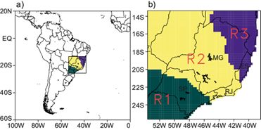
Fig. 1 (a) Area of study (rectangle) where the Southeast Region of Brazil (SEB) is encompassed. (b) Regions with homogeneous precipitation were determined from the cluster analysis. From south to north, we have R1, R2, and R3, respectively. The SEB states are identified on the map with the acronyms SP (São Paulo), RJ (Rio de Janeiro), MG (Minas Gerais) and ES (Espírito Santo).
According to Wilks (2006), in the cluster analysis, n grid points are considered n vectors with K dimensions each (K steps in time). In an initial moment, each vector is treated as a cluster (n clusters with K dimensions each). The next step is to join the two closest vectors to each other (with the smallest vector differences) to form a new cluster, and thus, the number of clusters becomes n-1. Ward’s minimum variance hierarchical method (Ward 1963) was employed to join the two closest clusters, aiming to minimize the sum of the internal vector distance variance for each cluster (W). The process of cluster merging (clustering) is repeated continuously until a given number of clusters is reached when the differences between the members of a specific cluster are minimized, and the differences between members of different clusters are maximized, or from another viewpoint, it is the creation of groups with homogeneous data.
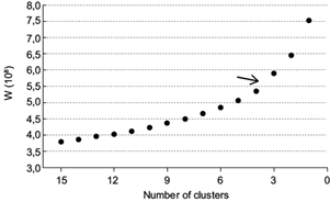
Some methods identify the stage in which the clustering process must be interrupted, a way of doing this for methods based on distance matrix is through the analysis of the graph showing the distance between clusters as a function of the clustering process stage (Wilks, 2006). Analogously, for Ward’s method, which is not based on the distance matrix, this step must be done by analyzing the graph showing W as a function of the number of merged clusters. The distances in the first cluster merge are usually small, and W increases slowly. This pattern tends to remain the same until the last stages of clustering, when clusters become more distant, and W increases faster, precisely because the differences between the clusters are more accentuated. Seen in W as a function of the number of remaining clusters scheme, this transition is identified by an important “jump” in the growth trend of W from one stage to another. Evaluating it by this subjective method, the moment to interrupt the process is exactly the moment when this “jump” occurs because it is the moment in which the distances between the clusters become considerably larger.
The graph shown in figure 2 presents W as a function of the number of clusters for the precipitation dataset of this work. Note that the figure only indicates the last 15 steps (from a total of 3100 initial clusters, or 3100 grid points within the study region), which is the progression of the clustering process between the time that there are 15 clusters and when there is only one cluster left. Note the continuous increase of W, from left to right of the graph, and the “jump” in the growth trend between points 4 and 3, indicated by an arrow. From this analysis, 3 clusters were found as representative. When these three groups of grid points are disposed of geographically, three regions with homogeneous daily precipitation data are identified, which is presented in figure 2. The regions were named, from south to north, R1, R2, and R3, respectively.
2.2.2 Determination of dry events
There is no universal index for determining droughts due to the various possible definitions for this phenomenon (Heim, 2002). We aim to determine drought events over a broad area and for a daily data series when there are no significant spatially or temporally precipitation episodes. For this task, two methods were employed: the consecutive dry days method (CDDM) and the variable threshold method (VTM). Van Huijgevoort et al. (2012) proposed this combination of two methods for the detection of hydrological drought events consistently and for regions with different runoff climatic regimes. Pampuch et al. (2016) adapted the two methods for meteorological droughts, taking this model as a basis for the script adopted here. According to Van Huijgevoort et al. (2012), in comparison with other methods widely adopted in the detection of droughts, such as SPI (Standard Precipitation Index) and PDSI (Palmer Drought Standard Index), the advantages of using these two methods are that knowledge of probability distributions is not needed, besides the creation of essential aspects of a drought event, such as frequency, duration, and severity. Also, even during summer shortage periods, the predominantly wet and tropical climate of SEB presents localized precipitation events. The CDDM makes a spatial assessment of droughts, where it is possible to identify dry periods in which such isolated rain events occur. On the other hand, VTM evaluates regional average rainfall as a whole.
The CDDM is simply based on a cumulative count of the dry days following some parameters. Here, the CDDM involves the following steps:
The days in which the precipitation was less than 1 mm were identified for each grid point. In theory, this threshold was supposed to be equal to 0 mm, but the value adopted here was due to the interpolated nature of the precipitation data.
If precipitation recorded at 75% of the grid points in a given region shows precipitation below 1 mm on a given day, that day is considered a “dry day.”
The consecutive “dry days” are counted until the day when the requirements in item 2 are no longer accomplished; that is, precipitation above 1 mm occurs in more than 25% of grid points, except for the condition listed in item 4.
It is allowed that up to one day, within a sequence of consecutive dry days, in a given region presents less than 75% of grid points with values lower than 1 mm, but at least 50% of grid points must meet this requirement.
The VTM shows whether the precipitation recorded on a given day characterizes an extreme dry value over the evaluated region as a whole. Unlike the CDDM, which uses the precipitation series at each grid point, the VTM is applied over the mean regional precipitation. The method utilizes a threshold to determine dry periods within a precipitation series, which is usually the 20th percentile, and it can be used either as a fixed or time-varying threshold (e.g.: seasonally, monthly, or daily) (Van Huijgevoort et al., 2012). A time-varying threshold is used to consider the seasonal precipitation cycle. For example, a daily-varying threshold considers a data series composed of every day of the year throughout the study period. In other words, for January 21st, we have a series of 37 data (37 days on January 21st throughout the 37 years of the data series).
Since a sample size of 37 would be too small to form a sample of appreciable size and without disregarding the local seasonal precipitation cycle, in this work, a time-varying threshold was chosen for a 10-day interval. Considering that the DJF is composed of 90 days (excluding the leap years), representing a total of 3330 days over the 37 years, nine series of 370 days each were created from this dataset. Therefore, the first series consists of the 1st to 10th of December days, the second one of 11th to 20th, and so on. To simplify, the nine daily precipitation data corresponding to the February 29th, present throughout the study period, were included in the last of the nine series described above, with the latter having 379 elements. The 20th percentiles were determined as the “dry thresholds” within each series, called P(20). A “dry day” is identified at the time that the daily precipitation of a given day falls below this threshold. A boxplot with the distribution of the precipitation data series over the 10-day intervals for each of the three sub-regions is shown in figure 3. The P(20) values in each interval are labeled and indicated by the red dots.
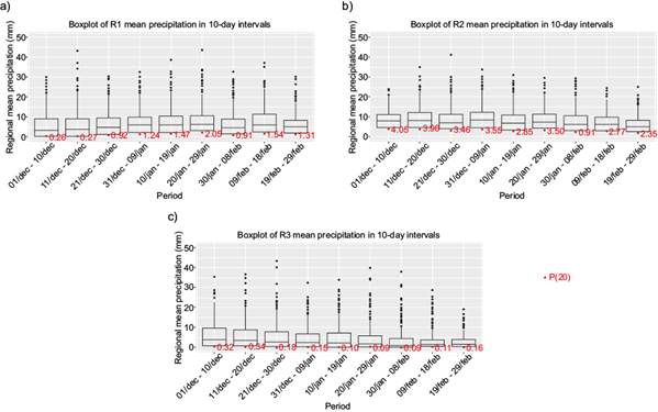
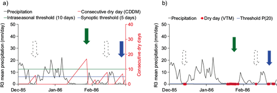
Fig. 3 (a) The Consecutive Dry Days Method (CDDM) and (b) the Variable Threshold Method (VTM) during the DJF 1985/86 period for the R3 region. The dark trace represents the regional mean daily precipitation in both figures. In (a), the moment that the accumulated dry consecutive days determined by the CDDM (red trace) exceeds the synoptic (blue line) or the intraseasonal (green line) thresholds, a dry event is identified by the CDDM. To validate the event, at least 50% of the CDDM event period must consist of dry days found by VTM (red dots) in (b). The arrows in the two figures indicate the synoptic (blue arrows) and intraseasonal (green arrow) dry events identified by the combination of the two methods, while the dotted arrow indicates an event that met the requirements of the CDDM but is not confirmed by the VTM.
In order to determine possible differences in the atmospheric and oceanic characteristics present during the dry events, which were identified by the methods at different timescales, two temporal thresholds were used. Firstly, dry events persisting for a minimum period of 5 consecutive days and a maximum of 9 consecutive days were called “synoptic dry events” (SDEs), while events lasting ten days or longer were named “intraseasonal dry events” (IDEs). In the combination of CDDM and VTM, a “dry event” is detected at the moment the CDDM requirements are met at the synoptic (5 days) or intraseasonal (10 days) dry threshold period, at the same time that it is confirmed at least 50% of “dry days” by the VTM along the same period determined by the CDDM. As previously mentioned, isolated rain events can occur in the CDDM, while VTM potentially inhibits them in part of the days (at least 50%), which reinforces and suits the method to the study region. In figures 4a and 4b, there is a graphical demonstration of how the CDDM acting along with the VTM detected dry events. The methods were applied separately to each homogeneous precipitation region determined by cluster analysis (R1, R2, and R3).
3. Results
3.1 Dry events statistics
As described in the introduction section, SEB is a vast region with somewhat different climatic regimes. Generally, summer is characterized as the rainy season, but with some differences within the region. These differences were the reason we divided the region into three sub-regions with more homogeneous characteristics in precipitation to analyze them better. Considering our precipitation dataset for the study period (DJF 1981/82 to DJF 2017/18), R2 (the central strip area in SEB) has the highest DJF average precipitation with 719 mm, while R1 (southernmost area) has 595.5 mm and R3 (northernmost area) has 393.3 mm. Some notion about how the mean regional precipitation varies seasonally in different aspects and within each sub-region can be obtained through the boxplot analysis in figure 3.
The total numbers of dry events (synoptic and intraseasonal) found by study region (R1, R2, and R3) between DJF 1981/82 and 2017/18 are shown in figure 5. Concerning intraseasonal dry events (IDEs), R3 was the region with the greatest number of occurrences (20 events), followed by R1 (7 events) and R2 (1 event). For synoptic dry events (SDEs), R1 recorded the highest number of cases (56 events), followed by R3 (37 events) and R2 (19 events). Despite the total number of events (SDEs plus IDEs) being greater in R1 (62 events) compared with R3 (57 events), if one considers the sum of “dry days” in such events, R3 has a total of 529 in comparison with 426 in R2. As shown in figure 3c, R3 has lower precipitation values most of the time than the other regions, resulting in more extended dry periods (especially IDEs). This also contributes to a decrease in the number of total events compared to the increase in the duration of dry events. It explains why R1 has more dry events than R3, despite not having the lowest climatological rainfall accumulations among the three regions.
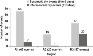
Fig. 5 The number of total synoptic (5 to 9 days) and intraseasonal (≥ 10 days) dry events were recorded in each of the homogeneous precipitation regions (R1, R2, and R3) from DJF 1981/82 to 2017/18.
The interannual variations of the DJF precipitation for each of the three homogeneous precipitation regions (R1, R2, and R3) are presented in figures 6a, 6c, and 6e (left side), respectively. A non-linear trend in these series, calculated using the LOESS regression (Cleveland et al., 1992), is drawn as a red line. For the same regions, respectively, in figures 6b, 6d, and 6f (right side), the interannual variations of the number of SDEs and IDEs identified by the CDDM and the VTM are shown. The correlation indexes of the interannual variation in the precipitation series with the interannual variations of the number of SDEs (r s ) and the number of IDEs (r i ) for each region are also presented. The figures are shown side by side, according to the region, to show the relationship between the dry events and the precipitation deficits.
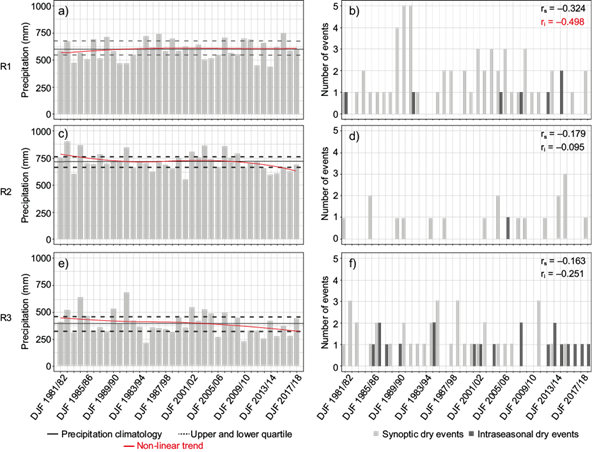
Fig. 6 Interannual variation of precipitation (left side) and a number of dry events (right side) between DJF 1981/82 to 2017/18 for regions R1 (a and b), R2 (c and d), and R3 (e and f). A red line on (a, c, and e) shows a non-linear trend (LOESS regression - Cleveland et al., 1992) in the interannual variation of precipitation series. Correlations indexes for the interannual precipitation series with the interannual number of SDEs (r s ) and with IDEs (r i ) in each region are shown in (b, d, and f). Values in red and bold denote a statistical confidence level above 95%.
The interannual variation of IDEs and SDEs is negatively correlated with the precipitation series in all the regions, as shown by the correlation indexes in the left-sided figures. Although the correlation is significant, above the 95% confidence level only for IDEs in region R1 (as indicated in bold in figure 6b). It demonstrates that the SDEs and IDEs identified here may not be the leading cause of shortage periods for greater timescales (monthly, seasonal and interannual), but they can partially explain them. A relevant number of years with precipitation deficits congruent with the occurrence of SDEs and IDEs can be found comparing the graphs. The dry summers of DJF 1991/92, DJF 2004/05, DJF 2011/12, and DJF 2013/14 were some of the driest seasons in R1 during the study period (Fig. 6a). At the same time, they showed at least 1 IDEs each (Fig 6b), besides presenting other SDEs. In R2, not many dry events were recorded over the sample time, but an increase in the SDEs coincides with the negative precipitation trend in recent years. In region R3, the quarters of DJF 1986/87 (2 SDEs and 2 IDEs), DJF 1994/95 (2 SDEs and 2 IDEs), and DJF 2012/13 (1 SDE and 2 IDEs) (Fig. 6f), three of the driest DJF over the data series (Fig. 6e), also presented expressive amounts of dry events when compared with other years as well as a recurrence of IDEs observed during the last years (Fig. 6f), which were drier than the climatological normal (Fig. 6e).
3.2 Mean fields and composites of anomalies
In this section, the mean fields and composites of several atmospheric and oceanic variables were analyzed for the periods of dry events using ERA-Interim reanalysis. Note that composites refer to mean values of anomalies, and mean fields do not use anomalies in their calculation. For each of the variables, the fields were made for SDEs and IDEs for each of the three homogeneous precipitation regions (R1, R2, and R3). Composites of Outgoing Longwave Radiation (OLR) and 500 mb geopotential height anomalies (Figs. 7 and 8) cover much of the southern hemisphere. The objective is to show, in addition to local atmospheric characteristics, wave train patterns associated with SEB dry events and possible sources. The composites and mean fields of remaining variables (Figs. 9 to 12) focus on local atmospheric and oceanic features, with the analysis domain confined to the surroundings of South America. It is important to emphasize that the mean fields and composites of anomalies show average atmospheric and oceanic behaviors during the dry events. Therefore, if one considers an isolated event, it may display different patterns than those presented here. Also, since only 1 IDE was registered in R2 with a duration of 12 days (small sample size), the composites and mean fields associated with that specific event are not shown.
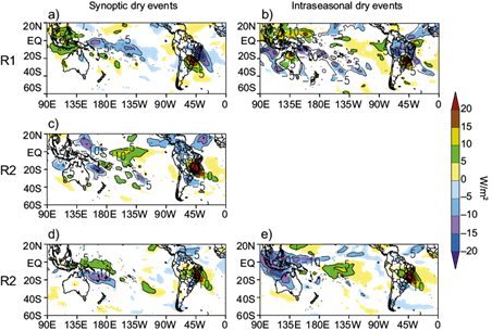
Fig. 7 Composites of outgoing longwave radiation (OLR) anomalies during the synoptic dry events in (a) R1, (c) R2, and (d) R3, and during intraseasonal dry events in (b) R1 and e R3. The shaded anomalies have a statistical confidence level above 95%.
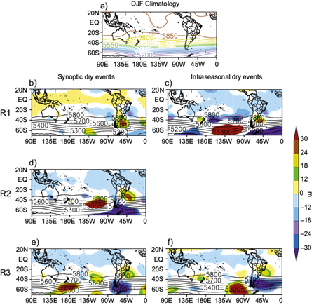
Fig. 8 (a) 500 mb geopotential height December-February (DJF) climatology for the period DJF 1981/82 to 2017/18. Mean fields of 500 mb geopotential (contours) and their respective anomalies (shaded) during the synoptic dry events in (b) R1, (d) R2, and (e) R3, and the intraseasonal dry events in (c) R1 and (f) R3. The shaded anomalies have a statistical confidence level above 95%.
Composites of OLR anomalies, encompassing an area covering the Pacific and Atlantic Oceans in the Southern Hemisphere, are shown in figure 7. Positive (negative) OLR anomalies are usually associated with lower (greater) cloud cover values and negative (positive) precipitation anomalies. All fields in figure 7 show significant positive OLR anomalies over the regions reporting dry events. When considering the South American continent, some OLR patterns can be observed simultaneously with the dry periods over the study regions. A noticeable pattern is a meridional precipitation dipole, which varies in location according to the region of interest. In R2 SDEs (Fig. 7c), this pattern is located between the central-eastern region of Brazil (positive OLR anomalies) and SESA (negative OLR anomalies). In the R1 and R3 cases (Figs. 7a, 7b, 7d, and 7e), this dipole is practically between such regions, plus part of southern Brazil (in the R1 pole) and part of northeastern Brazil (in the R3 pole). This pattern is prevalent during drought events in the central-eastern portion of Brazil, and it has been reported in many works (e.g., Nogués-Paegle and Mo, 1997; Barros et al., 2000; Robertson and Mechoso, 2000; Ferraz, 2004; Castro-Cunningham and De Albuquerque-Cavalcanti, 2006; Muza et al., 2009; Grimm and Zilli, 2009; Gonzalez and Vera, 2014). Another recurring pattern, which was not observed only in R1 SDEs, is the negative OLR anomalies in the Intertropical Convergence Zone (ITCZ) region. Considering the equatorial Pacific band, for R2 SDEs, R3 SDEs, and R3 IDEs (Figs. 7c to 7e), is verified significant negative OLR anomalies over Indonesia and positive anomalies over the central part. For R1 cases (Figs. 7a and 7b), negative OLR anomalies are observed more in the central-western equatorial Pacific. It is worth mentioning that such regions of anomalous convective activity over the equatorial Pacific commonly act as a source of teleconnections patterns that may contribute to the dry events over SEB, although it is not the scope of this work to investigate that further.
The 500 mb geopotential height DJF climatology is shown in figure 8a. The same variable mean fields (contours) and their respective anomalies (shaded) for the dry events are shown in figures 8b to 8f. For this variable, it was decided to place the climatology field for a clearer notion of how some atmospheric systems behave on average during dry events in relation to the climatological normal. In all the cases, a positive anomaly is noticed south of the region of the dry events. This configuration makes the approximation of transient disturbances, which are usually associated with the precipitation over the SEB, difficult. For SDEs and IDEs in R1 (Figs. 8b and 8c), a positive anomaly along the Argentine coast (shaded in warm colors) is verified, related to a ridge over the entire southern portion of South America (isohypses) at the same time that it is possible to observe a negative anomaly pole over the SEB coast (shaded in cool colors) related to a trough over this location (isohypses). This pattern can be produced by passages of slow transient systems in the synoptic scale. It is also possible that northern-shifted SACZ episodes could also contribute to that in both timescales. In these possible cases of SACZ, the ridge and the trough associated with the SACZ are more amplified than in the usual cases and with a slight zonal displacement of the trough towards the central Atlantic Ocean, which corresponds to the reallocation of the greatest precipitation region to the north, on the south portion of Northeast region of Brazil.
In contrast, dry conditions are verified in the southern half of the SEB and southern Brazil (as seen in Figs. 7a and 7b). For R2 and R3 cases (Figs. 8d o 8f), a blocking ridge is approximately centered between the coasts of Brazil’s southern and southeastern regions. Although with less intense signals, this pattern is similar to those found for the 2014 and 2015 dry events (e.g., Seth et al., 2015; Coelho et al., 2016; Cavalcanti et al., 2017). Further, good similarity exists with the events of those years between the wave train pattern found for SDEs, in R2 and R3 and IDEs in R3 (Figs. 8d to 8f). The wave train extends from the central Pacific Ocean to the South American continent with minor differences between the cases. It displays a trough over the central Pacific subtropics, a ridge over the southwest of Chile, another trough over the southwest Atlantic Ocean, and the blocking ridge over the southern and southeastern Brazilian coasts. This feature, plus the convection over Indonesia for the same class of events (Figs. 7c to 7e), suggests that many times the origin of these events is similar to the teleconnection pattern identified for the 2014 and 2015 dry summers (e.g., Coelho et al., 2016; Rodrigues et al., 2019; Finke et al., 2020).
Now, looking specifically at South American atmospheric conditions, anomalous patterns with some resemblances to those observed in the 500 mb geopotential height fields are also observed in the mean sea level pressure (MSLP) fields (Figs. 9b to 9f), demonstrating the barotropic nature of the anomalies. For events in R1 (Figs. 9b and 9c), it is verified a prevalence of positive (negative) anomalies over the extratropics (tropics) in South America. In contrast, the opposite is noticed in R3 (Figs. 9e and 9f). It denotes a South Atlantic Subtropical High (SASH) inclined and extended to the southwest for events more to the south (R1 cases) and inclined to the northwest in northern cases (R3 cases) when this SASH’s continental approach to the South American continent contributes to the atmospheric stabilization over the regions of dry events.
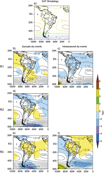
Fig. 9 (a) Mean sea level pressure (MSLP) December-February (DJF) climatology for the period DJF 1981/82 to 2017/18. Mean fields of MSLP (contours) and their respective anomalies (shaded) during the synoptic dry events in (b) R1, (d) R2, and (e) R3, and the intraseasonal dry events in (c) R1 and (f) R3. The shaded anomalies have a statistical confidence level above 95%.
Figure 10a it is shown the 200 mb wind (streamlines), magnitude (contours), and divergence (shaded) DJF climatology, while the mean fields for the dry events in each region and event class are presented in figures 10b to 10f. Upper-tropospheric circulation exhibits a very characteristic pattern during the rainy season of the tropical portion of South America, which occurs on average between mid-spring and early autumn and encompasses our study period. From the DJF climatology (Fig. 10a), it can be seen two typical systems of the tropical upper troposphere: The Bolivian High (BH), anticyclonic circulation due to the grand release of latent heat associated with tropical convection (Lenters and Cook, 1997), centered over Bolivia; and the Atlantic trough (AT), that is observed along the coast of northeastern Brazil, which at times becomes a closed cyclonic circulation, called the upper tropospheric cyclonic vortex of the Brazilian Northeast (VBNE). According to Ferreira et al. (2009), the most favorable regions for upward (downward) movements in the system composed of BH-VBNE or BH-AT circulations are the locations where the most expressive diffluences (confluences) of the flow are found. As mentioned before, in both R1 cases (Figs. 10b and 10c), the dry periods seem to be associated with a post-frontal situation or a northern-shifted SACZ condition. A second trough is observed over a subtropical latitude near the southern coast of Brazil, beyond the AT at tropical latitudes, resembling a typical SACZ trough, also verified in the mid-troposphere (Figs. 8b and 8c). Divergence is verified downstream of this southern trough as well as over a broad area of diffluence between the BH and AT systems in the northern part of Brazil, whereas upstream of the southern trough, a convergence is observed over an area encompassing southern Brazil and the region corresponding to R1 (southern SEB). In R2 and R3 events (Figs. 10d to 10f), the system, composed of BH-AT (SDEs in R3) and BH-VBNE (SDEs in R2 and IDEs in R3), is displaced southwest of its climatological position. The BH is centered approximately over southern Bolivia, while the AT or VBNE acts near the SEB’s northern and southern parts of the Brazilian Northeast. For such events, both the AT and the VBNE have a slope towards the eastern part of Brazil. It can be seen that the regions with dry events are generally located under confluence areas of the BH-VBNE or BH-AT systems, just to the west of VBNE or AT location, and present negative values of divergence (i.e., convergence) in the upper troposphere. This atmospheric condition leads to downward movements over these regions, contributing to the persistent stable weather associated with the dry events. The VBNE core lies near SEB by itself (e.g.: SDEs in R2 and IDEs in R3), south of its climatological position, which may contribute to the atmospheric stabilization over such regions because of the typical subsidence within this system (Ferreira et al., 2009). Looking at the other areas in the South American continent, in all cases, we see a region of expressive diffluence in the flow of the BH-VBNE or BH-AT systems in the north of Brazil, where there are large areas of positive values of divergence, which correspond to the vast area of convection over that region. Another point of diffluence is identified over southern Brazil and SESA for events in R2 and R3 (Figs. 10d to 10f), showing positive values of divergence and, hence, rainfall conditions over that place (see Figs. 7c to 7e). In this region, the upper troposphere divergence may also be increased by being located in an equatorial entrance of a reinforced Upper Tropospheric Jet (UTJ) (see contours in Figs. 10d to 10f).
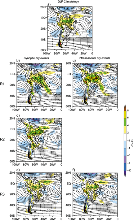
Fig. 10 (a) 200 mb wind (streamlines), magnitude (shaded), and divergence (contours) December-February (DJF) climatology for the period DJF 1981/82 to 2017/18. Mean wind fields (streamlines), magnitude (shaded), and divergence (contours) during the synoptic dry events in (b) R1, (d) R2, and (e) R3, and the intraseasonal dry events in (c ) R1 and (f) R3.
Figure 11 shows wind and specific moisture anomalies at 850 mb. In the R1 events (Figs. 11a and 11b), a cyclonic anomaly is verified near the SEB coast, which contributes to reinforcing the western wet flux over the northern SEB and northeastern Brazil and inducing an anomalous drier eastern flux over the southern part of SEB, where R1 is located. The presence of an anomalous anticyclone is verified near the southern and southeastern coast of Brazil for events in R2 and R3 (Figs. 11c to 11e). Such circulation is associated with the intensification and displacement of SASH towards the east coast of Brazil. In all the R2 and R3 cases, the associated circulation intensifies the South American Low-Level Jet (SALLJ) east of the Andes, channeling the wet stream towards southern Brazil and SESA. One noticeable aspect common to all anomalous wind fields is the eastern component with associated moisture deficit over the study regions, as is also verified in Muza et al. (2009) in a study about dry events variability on an intraseasonal and interannual scale. This anomalous eastern component is responsible for weakening the northwestern wet climatological flow over each study region and contributes to the shortage periods.
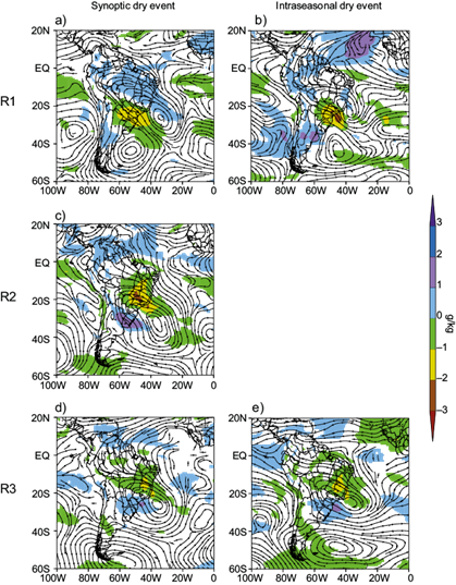
Fig. 11 Composites of 850 mb wind (streamlines) and the specific moisture (shaded) anomalies during the synoptic dry events in (a) R1, (c) R2, and (d) R3, and during the intraseasonal dry events in (b) R1 and (e) R3. The shaded anomalies have a statistical confidence level above 95%.
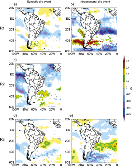
Lastly, the SST anomaly fields are shown in figure 12 . According to Jorgetti et al. (2014), the pattern with a negative anomaly strip between the SEB coast extending zonally over the south Atlantic, as seen for the R1 cases (Figs. 12a and 12b), is typical of northern-shifted SACZ events. It contributes to the origin and the maintenance of the rainy continental band in a northward position, then contributes to the occurrence of the dry events in the southern SEB. The cold anomalies near the southern SEB coast intensify the continent-ocean temperature gradient, characteristic of summer, then favoring an easterly drier anomaly flux (as seen in the Figs. 11a and 11b), holding the rainfall pattern to the north (Doyle and Barros, 2002; Jorgetti et al., 2014). For R2 and R3 events (Figs. 12c to 12e), the SST anomaly pattern resembles the typical case found associated with dry events over SEB (Coelho et al., 2016; Pampuch et al., 2016; Pattnayak et al., 2018; Rodrigues et al., 2019), as well as the case of southern SACZ events (Jorgetti et al., 2014). A strip of positive SST anomalies near SEB is verified, which probably responds to the increased incident radiation and negative anomalies of latent heat flux, as shown by Rodrigues et al. (2019). Over mid- and high-latitudes, the main SST anomaly patterns are clearly associated with the dynamic atmospheric conditions shown in the previous figures and mainly respond to them. We compare the SST anomalies with the 500 mb geopotential height anomalies (Fig. 8). Under areas with negative anomalies of 500 mb geopotential height and MSLP, there is usually a greater instability of the environment and a greater cloud cover value, and a consequent decrease in SST due to the smaller amount of incident radiation. The opposite, positive SST anomalies, occur under the areas of positive anomalies of 500 mb geopotential height, where there is a greater atmospheric stabilization, a lower cloud cover value, and a greater amount of incident radiation. As can be seen, for events in R1 (Figs. 12a and 12b), the SST anomalies pattern has almost inverted signals with respect to the other two regions (Figs. 12c to 12e), and the main cause seems to be the configuration of the mid and upper-tropospheric wave train pattern for such cases, which also has signals practically inverted to each other (see Fig. 8). An SST anomaly tripole pattern along the eastern coast of South America, which is more evident in R1 SDEs and R3 IDEs (Figs. 12a and 12e), is also worth noting. It is verified negative (positive) SST anomalies in the central pole and negative (positive) anomalies in the north and south poles for the R1 cases (R3 cases). These patterns are similar to those found by Pampuch et al. (2016) for dry periods in similar areas over the SEB, occurring in the autumn, winter, and spring seasons.
4. Conclusion
This work characterized the atmospheric and oceanic patterns of dry events occurring in the Southeast Region of Brazil (SEB) during the austral summer, the season with the greatest rainfall accumulations in the region. Thirty-seven summers (DJF) between 1981/82 and 2017/18 of daily precipitation data were analyzed to identify dry events in the SEB. Because of the region’s broad area, with precipitation regimes varying in time and space, three sub-regions (R1, R2, and R3) with homogeneous precipitation characteristics were identified within the SEB using the cluster analysis method. The R1 region, further south, encompasses the majority of the Brazilian state of São Paulo and small parts of bordering states. R2 region covers a central strip extending diagonally between the Brazilian states of Goiás and Rio de Janeiro. R3, further north, is composed of northern Minas Gerais, Espírito Santo and southern Bahia.
The dry events identification was performed by the consecutive dry days method (CDDM) and the variable threshold method (VTM), applied together to the daily precipitation data. The identification was made separately for the three homogeneous precipitation regions (R1, R2, and R3). The dry events were classified according to their duration as synoptic dry events (SDEs) (between 5 and 9 days in duration) and intraseasonal dry events (IDEs) (10 or more days in duration). The drier the region is, the greater the number of IDEs found, with the R3 region (393.3 mm of DJF average) recording 20 events, R1 (595.5 mm) reporting seven events, and R2 (719.0 mm) recording one event. For SDEs, R1 had the greatest number of events recorded (56 events), followed by R3 (37 events) and R2 (19 events). As expected, interannual variation in precipitation is negatively correlated with the interannual variation of dry events, with a significant value occurring only for R1 IDEs, which can indicate a partial explanation of shortage periods on longer timescales by the dry events identified here.
Considerable differences in atmospheric and oceanic features are seen between dry events taking place in the southern (R1) and central northern (R2 and R3) parts of SEB, while no significant differences were found according to event duration class (SDEs and IDEs). Events in R1 exhibited a pattern that could be produced either by a frontal system with a high pressure behind (over R1) or by a persistent SACZ episode but displaced northward, this last one, especially for IDEs cases. SST cold anomalies over subtropical Atlantic seem to contribute to maintaining a northern-shifted SACZ pattern and, therefore, a drier condition over southern SEB in such cases. For central and northern dry events, in R2 and R3 regions, the atmospheric and oceanic patterns resemble those verified in 2013/14 and 2014/15 summer, with an anomalous blocking high acting close to the SEB coast and a significant strip of positive SST anomalies below.
Other interesting atmospheric conditions over the South American continent, which were associated with the dry events, deserve to be mentioned. A precipitation dipole, which varies its location meridionally according to the homogeneous precipitation region, is verified on the OLR anomaly fields for all study regions (R1, R2, and R3) and in both classes of dry events (SDEs and IDEs). This dipole was characterized by a drier and a wetter pole, which were approximately located between the southern part of Brazil (dry pole) and the northeastern part of Brazil (wet pole) in R1 cases, SEB (dry pole) and SESA (wet pole) in R2 cases, and the opposite of R1 cases in R3. The DJF climatological low-level flow over the SEB is from the northwest, which commonly brings humidity from the Amazon region. During the dry episodes, the flow presented an eastern anomaly component that represents a weakening of this climatological northwestern flow; therefore, a decrease in humidity over the SEB is seen. This eastern component corresponds to the southern part of an anomalous cyclonic circulation for R1 events, bringing an anomalous moist western flux over northeastern Brazil in its northern flank. For the cases in R2 and R3, the eastern component is the northern part of an anomalous anticyclonic circulation that, in its turn, provides a wetter flux over southern Brazil and SESA. For almost all dry events cases, negative OLR anomalies were also noticed in the Intertropical Convergence Zone (ITCZ) region. A SASH intensification and shift towards the eastern coast of Brazil was identified in the R2 and R3 events. Furthermore, in the upper troposphere, the system composed of BH-VBNE (BH-AT in some cases) is generally displaced south of its climatological position in R2 and R3 events.
This research is important for weather and climate forecasts because it suggests general atmospheric and oceanic patterns linked to extreme dry events. A further investigation on how some oscillations of different timescales may contribute to originate the dry periods over the different parts of SEB, like teleconnections patterns, the Madden-Julian oscillation or the El Niño Southern Oscillation, as well as the SST patterns associated with them, will be the focus of future work.

