


 nueva página del texto (beta)
 Inglés (pdf)
 Artículo en XML
 Referencias del artículo
 Enviar artículo por email
 Citado por SciELO
  Similares en
SciELO
Similares en
SciELO 
 Permalink
1. Introduction
There is ample evidence on the relationship between ambient Particulate Matter (PM) concentration and mortality, morbidity, and other health-related effects. According to a study made by the World Health Organization (WHO) in 2014 (WHO, 2017), 92% of the world population was living in places that did not meet the WHO’s air quality standards, and in 2012 air pollution caused 3.7 million premature deaths around the world1. In relation to the health effects of PM, the Technical Report of the European Regional Office of WHO (2013) concludes that there has been increasing evidence on the short and long-term consequences of PM exposure on health, mortality, and morbidity.
Many studies interpret the association between PM concentration and mortality as the response in a cluster of people with fragile health, for example, individuals with chronic cardiac or respiratory diseases and the elderly (US-EPA, 1996), which suggests that this association reflects the shortening of life expectancy by a few days. This represents, essentially, the mortality displacement effect, and it is the dominant interpretation of the strong and systematic association between air pollutants and mortality.
We think that the severity of environmental problems requires a new approach to environmental public policy and stress the need to quantify the shortening of life expectancy implied by the evidence relating air pollution to mortality. To achieve this objective, we applied the Murray and Nelson (2000) model, which allows us to plot the number of individuals in the at-risk population over time using the mortality data observed, as well as to estimate the hazard rate and life expectancies among the at-risk population. Just like them, we believe that understanding the dynamics of the at-risk population will improve our understanding of the relationship between pollution and health.
In this study, we explore whether socioeconomic differences across municipalities of the Metropolitan Area of the Valley of Mexico (MAVM) have an effect on the health risks associated with air pollution within the framework of environmental justice. According to Schlosberg (2013), environmental justice in general addresses inequality in the distribution of negative effects of environmental damage, and therefore some population groups are at higher environmental risk than others due to their unequal socioeconomic and locational characteristics. In these terms, environmental justice is just one of the many faces of social inequality. In our work, we adopt the traditional concept of environmental justice, namely, the association of a geographically localized relation between socially disadvantaged populations and environmental pollution.
There are different conceptions of environmental justice. According to Menton et al. (2020), the most widely accepted considers the following four dimensions: (1) distributional justice, that is, the fair distribution of environmental costs and benefits, the allocation of material goods or the distribution of social standing; (2) recognitional justice, recognition of, and respect for, the difference; (3) procedural justice, the fair and equitable institutional processes of a State, and (4) the capability approach, the recognition that justice takes into consideration the distribution of goods but also, and more importantly, the way those goods enhance the capacities of each person to lead a life worth living.
In this paper we study the relation between air pollution and the unequal socioeconomic characteristics of the population that live in three different municipalities in the MZVM. We are interested in studying the association of those unequal conditions on the life shortening effects of air pollution upon the most vulnerable population who live in conditions of social inequality. Within the environmental justice framework, there is a very new and interesting approach to the study of the joint effects of inequality and air pollution on heath. This new line of research is less interested in the direct and indirect effects of income inequality on health due to air pollution. Particularly, in one of the first studies within this approach Hill et al. (2019) ask if a specific localized population (in this case that of USA states) is especially vulnerable to similar levels of air pollution (Hill et al., 2019). They argue that income inequality has a multiplier effect based on the following three theoretical principles:
Power: income inequality tends to concentrate economic and political power and as a consequence, the design of environmental policy in favor of the status quo
Proximity: income inequality tends to spatially segregate the socially vulnerable population in certain parts of the city or the territory.
Psychology: multiplier effect of psychological factors associated with social disadvantage in general and income inequality in particular generate a diversity of stressful situations that increase the cumulative burden of chronic stress and life events or the so-called allostatic load (Guidi et al., 2021).
The authors find that air pollution has a negative effect on life expectancy in those USA states with higher income inequality as measured by the income share of the top 10%.
A more recent study by Jorgenson et al. (2021) within the above-mentioned approach following Hill et al. (2019) asks if the effect of air pollution as measured by the concentration of PM2.5 on life expectancy is greater in nations with higher levels of income inequality. Jorgenson et al (2021) tend to confirm their hypothesis.
Therefore, understanding exposure variations among subpopulations is important for risk management and environmental justice. Environmental health policy must seek not only to reduce population average risk but also to ensure that specific subpopulations are not unduly burdened relative to the overall population. Policymakers concerned about environmental justice argue that communities who are segregated in neighborhoods with high levels of poverty and material deprivation are also disproportionately exposed to a physical environment that adversely affects their health and well-being. They have also noted that groups with low socioeconomic status become concentrated, centralized, and isolated in abandoned inner-city cores where employment opportunities are few and where communities are clustered around industrial sites, undesirable land use, and transportation corridors that pose a significant health hazard (Pulido et al., 1996).
In terms of social and economic inequality, it has been documented the importance of economic and political power and their negative effects on environmental justice and thus on life expectancy (Romero et al., 2013; Hill et al., 2019). This is particularly true in urban areas where economic and political elites concentrate and live, in parts of the cities equipped with the best urban infrastructure, the higher density of green areas and open spaces, and, in general, with a higher supply of urban amenities including those related with a higher quality of life. As Romero et al. (2013) argued, intra-urban differences in temperature are related to affluence, and as poorer municipalities tend to be more densely settled and have a smaller proportion of green spaces, they are exposed to higher levels of air pollution. Furthermore, some studies have found that poorer neighborhoods are exposed to higher levels of air pollution and that the less financial, human, natural or social resources or assets people have, the more vulnerable they are to the various hazards they face (Moser and Satterthwaite, 2010).
The study of environmental justice is particularly important for MAVM due to several reasons. First, there is no explicit recognition of environmental justice in any of the different laws, local and federal, related to the environment2. Consequently, the design of environmental public policies does not consider the possibility of differences in environmental risks according to the socioeconomic conditions of the population3.
Second, like all Mexican urban areas the MAVM has two important characteristics for the study of pollution-related mortality from the environmental justice point of view:
It is deeply segregated both socially and spatially and this phenomenon has been increasing throughout the years (Monkkonen, 2012; Sánchez, 2012a, b; Rubalcava and Schteingart, 2012). There is also evidence that there is spatial segregation according to the distribution of green areas in Mexico City (González, 2020). Furthermore, urban segregation has positive effects on socioeconomic inequalities (Reardon and Bischof, 2011).
According to the Consejo Nacional de Evaluación de la Política de Desarrollo Social (National Council for Evaluation of Social Development Policy; CONEVAL), about 34.4% of the MAVM population is living in poverty conditions and elder people are even more segregated (Garrocho y Campos, 2016).
Third, there is evidence that in Mexico there is a systematic relation between social inequalities in health, including health care, and socioeconomic inequalities (Barraza-Lloréns et al., 2013). Therefore, we think that it is important to consider this fact given the close relationship between environmental justice and health inequality (Brulle and Pellow, 2005; Wakefield and Baxter, 2010).
Fourth, there are a few studies for the MAVM that explore whether socioeconomic differences have an effect on the relationship between health risks and pollution. Romero et al. (2013), for example, analyzed the origin of health risk among the inhabitants of Bogotá, Mexico City, and Santiago. These authors concluded that “[W]hile proponents of the environmental justice perspective may expect that spatial differences in environmental hazards overlap with socioeconomic characteristics of human settlement, our results suggest that the association between levels of air pollution and social vulnerabilities do not always hold within the study cities.” Their findings also suggest a kind of “boomerang effect”, i.e., a situation that affects both rich and poor people. Even though we agree that pollution affects rich as well as poor inhabitants, our proposal shows some evidence in favor of environmental justice.
Finally, we think that environmental justice, both as analytical framework and as a principle to design and evaluate environmental policies, provides the right perspective to face some of the most urgent environmental problems that Mexican local governments need to solve. The environmental justice approach allows considering the different factors that affect environmental problems: an environmental policy must be a health, social, urban, and transport policy as well.
Accordingly, we hypothesize that the association between PM concentration and mortality in unequal socioeconomic municipalities of the MAVM depends on socioeconomic differentiation. To test this hypothesis, we selected three municipalities of the MAVM, with high, middle, and low-income levels. From a public health viewpoint, the arguments for taking a municipality approach to examining the relationship between socioeconomic status, environment, and health disparities are twofold. First, the theory suggests that it is appropriate to assess environmental health disparities at the territorial level because economic trends, transport planning, and industrial clusters tend to be regional in nature. In fact, zoning, facility location, and urban planning decisions tend to be local (Morrelo-Froch et al., 2002). Second, studies examining how health disparities play out regionally could provide information to propose public health policy initiatives that improve living conditions among diverse communities, particularly for those communities whose illnesses relate to poor environmental conditions.
To our knowledge, our work is the first study for the MAVM case that estimates and plots the unobserved at-risk population as well as its hazard rate and life expectancy using the Kalman filter. As a result, it was possible for us to show inconsistency with the displacement hypothesis for the high-income municipality. We provide evidence of an impact not only to the at-risk population but also to the generally healthy individuals exposed to high levels of air pollution for a sufficient amount of time to develop chronic conditions and enter the at-risk population. We found that low socioeconomic municipalities tend to have high vulnerability to air pollution, that is, a given exposure level may cause greater than average health reduction for these groups. The socioeconomic disparities between municipalities partially explain why we observe a lower hazard rate with high variability in the wealthy municipality as compared to the higher hazard rate with low variability in the poor one. The lower hazard rate of the wealthy municipality extends life span and allows people to stay longer in the at-risk group, thus increasing the size of that population, as compared to the at-risk population in the poor municipality, whose individuals have a lower life expectancy.
We organized the paper into four additional sections besides this introduction. Section 2 describes the climatic, atmospheric, and socioeconomic conditions of our selected municipalities and highlights the high disparities among them. It also describes and characterizes the data applied to explore health risks. Section 3 presents the model we used to estimate the relationship between PM concentration and mortality. We propose a state-space model that allows us to estimate the number of individuals of the population at risk, the life span of individuals in that group, as well as the effect of changes in air quality over the life span. The empirical analysis is carried out in section 4, while section 5 presents some discussion and concluding remarks.
2. Study area and data
2.1 Municipalities
The MAVM, with a population of nearly 21 million people, expands over three states (Mexico City and the states of Mexico and Hidalgo). It comprises the 16 municipalities of Mexico City, 59 municipalities of the state of Mexico, and one municipality of the state of Hidalgo. In 2010, according to CONEVAL (2014), almost 35% of the total population was in poverty conditions.
The MAVM is located in an elevated basin surrounded by mountains on the east, south, and west, with a narrow gap to the south-southwest and a broad opening to the north. Pollutants are trapped within the basin by mountains and term inversions, which are frequent during winter. In addition, the high altitude makes combustion sources less efficient. The tropical latitude (19º 25’ N) and the high altitude (2240 masl) make sunlight less intensive than in lower elevation, higher latitude cities (Molina and Molina, 2004). The MAVM’s climate is generally dry, but thunderstorms are frequent and intensive from June through October. Winter is slightly cooler than summer. Since specific humidity, temperature, and wind speed acted as cleaners of PM for the atmosphere, the safest period for the MAVM in terms of PM emissions is precisely from June through October.
We used diverse criteria in the selection of the three municipalities to evaluate if health risks related to air pollution are socioeconomically differentiated. In order to examine health risks, we needed to gather, validate, and analyze data on air pollution, local temperature, and socioeconomic vulnerability. Álvaro Obregón, Iztapalapa, and Naucalpan de Juárez were those municipalities having the complete data set to carry out our study.
With a population of 1 815 768 inhabitants, according to data from the 2010 census, Iztapalapa is the most populous municipality both in the MAVM and the whole country. Over 92% of Iztapalapa’s territory is urban, whil 43.8 and 45% of Álvaro Obregón’s, and Naucalpan’s territory, respectively, was urban. Regarding industrial land use, 3.0, 3.2, and 0.7% of the territory of Iztapalapa, Naucalpan de Juárez, and Álvaro Obregón, respectively, is used for industrial activities.
Being the most populous municipality, Iztapalapa has very demanding transportation requirements. Almost all means of transportation in this municipality operate through various roadways on both public and private vehicles. The most important road in Mexico City goes through this area. Every day, a total of about 80 000 vehicles moves through this route, making it the second busiest in the MAVM. According to the 2017 origin-destiny survey (INEGI, 2017), Iztapalapa was the origin of 971 765 daily trips and the destiny of 970 135 daily trips.
The most relevant economic activities in Iztapalapa are manufacturing and commerce. The three largest sectors of retail sales are street markets, flea markets, and street vendors who flagrantly violate sanitation and environmental laws. Food processing, tobacco products, metals, machinery, surgical equipment, paper and printing, and textiles are also included.
Naucalpan de Juárez is a municipality in the state of Mexico, northwest of Mexico City, which according to the 2010 census had a total population of 833 779 inhabitants. Its subsoil is highly polluted, mainly because of the Bordo Poniente landfill and the sagging of the subsoil due to the overpumping of groundwater and the jettison of untreated wastewater. Furthermore, other small businesses (e.g., brick making operations, public restrooms, and restaurants) blatantly infringe sanitation and environmental laws and increase the pollution in the municipality. Nevertheless, vehicles are the origin of 70% of the air pollution; in 2017, they were the origin of 442 063 daily trips and the destiny of 447 799 daily trips (INEGI, 2017).
The most stringent environmental regulations promoted by a growing middle class have been enacted and enforced, which has caused the relocation of several highly polluting industries to the north and west of the MAVM. Industries that have left Naucalpan de Juárez include the metal, cement, and glass industries, as well as others using a large quantity of energy. About 20% of the manufacturing facilities have closed their doors and six industrial parks are empty.
Álvaro Obregón encompasses a large portion of the southwest area of Mexico City. According to the 2010 census, it had a total population of 727 034 inhabitants. The municipality occupies 7720 ha, of which is 66.1% urban land and 38% is considered protected land. Services-including financial services-make up the largest segment of the municipality economy, accounting for 75.6% of gross domestic product and employing about 76.14% of the workforce. This municipality is an important economic center and in 2017 it was the origin of 552 720 daily trips and the destiny of 555 629 daily trips (INEGI, 2017).
Table I shows that, while variations in the average daily temperature in any of these municipalities are not high, variations in daily average pollution are. For example, the daily average level of PM104 range between 6.88 and 115.32 µm m-3 in Álvaro Obregón, while for Iztapalapa the daily average level ranges between 7.00 and 268.00 µm m-3. Large differences in pollution emissions will imply different hazard exposures to those municipalities. According to impact studies about urban vulnerability, the risks of adverse health impacts depend on two different factors. The first one is related to the origin of the hazard for urban populations, while the second is related to the socioeconomic conditions influencing the exposure, the sensitivity and the responsiveness to risk, as well as its effects on health, all of which may reflect inequalities in the access to services and well-being systems. Therefore, it is important to explain the current environmental and socioeconomic situation of these municipalities.
Table I Environmental and socioeconomic features of the study municipalities.
| Álvaro Obregón | Naucalpan de Juárez | Iztapalapa | |||||||
| Min. | Mean | Max. | Min. | Mean | Max. | Min. | Mean | Max. | |
| PM10 (daily average in µg m-3) | 6.88 | 38.79 | 115.32 | 6.33 | 45.14 | 137.27 | 7.00 | 54.36 | 268.00 |
| Daily average temperature (ºC) | 5.80 | 16.30 | 23.94 | 5.44 | 16.24 | 25.82 | 7.00 | 16.70 | 25.00 |
| Non-accidental mortality | 1.00 | 9.28 | 25.00 | 1.00 | 9.91 | 24.00 | 5.00 | 20.00 | 47.00 |
| Cardiovascular and respiratory mortality | 0.00 | 2.56 | 11.00 | 0.00 | 2.53 | 10.00 | 0.00 | 5.06 | 21.00 |
| Years | |||||||||
| 2000 | 2005 | 2010 | 2000 | 2005 | 2010 | 2000 | 2005 | 2010 | |
| Population | 687,020 | 706,567 | 727,034 | 858,711 | 821,442 | 833,779 | 1,773,343 | 1,820,88 | 1,815,786 |
| Poverty | |||||||||
| Annual per capita income (PPP USD) | 14,816 | 13,651 | 20,177 | 13,583 | 14,171 | 20,112 | 10,078 | 10,481 | 16,126 |
| PWNM2S | 43.07 | 33.24 | 23.64 | 47.11 | 38.72 | 28.02 | 50.29 | 38.82 | 36.04 |
| Gini coefficient | na | na | 0.442 | na | na | 0.454 | na | na | 0.409 |
| Dwelling | |||||||||
| % all home appliances | 17.18 | na | 29.78 | 16.01 | na | 25.85 | 8.22 | na | 22.36 |
| % home ownership | 73.63 | na | 65.52 | 67.77 | na | 59.75 | 75.78 | na | 66.95 |
| Socio-demographics | |||||||||
| PRM18BD | 131.82 | 178.77 | 210.50 | 112.87 | 153.70 | 163.38 | 83.52 | 117.73 | 138.71 |
| % people where the head-household is indigenous | 2.58 | 1.69 | 1.83 | 4.93 | 4.35 | 5.63 | 3.94 | 2.95 | 3.88 |
| Gender and household composition | |||||||||
| % female labor force | 39.16 | 41.93 | 35.15 | 37.23 | 35.01 | 38.44 | |||
| % female-headed household | 23.61 | 26.93 | 29.38 | 20.00 | 23.20 | 24.87 | 22.27 | 26.09 | 29.00 |
| Average person per household | 4.15 | 3.87 | 3.68 | 4.18 | 3.94 | 3.82 | 4.33 | 4.09 | 3.91 |
| Percentage of households with more than seven members | 5.89 | 4.40 | 3.46 | 5.45 | 4.10 | 3.45 | 6.81 | 5.39 | 4.31 |
| Employment | |||||||||
| % unemployment | 1.76 | na | 4.43 | 1.37 | na | 4.51 | 1.66 | na | 5.05 |
| % informally employed | na | na | 26.13 | na | na | 24.06 | na | na | 28.03 |
| Health | |||||||||
| % population without public healthcare | 47.12 | 40.57 | 30.03 | 44.79 | 43.56 | 41.60 | 51.31 | 50.51 | 38.30 |
| Infant mortality rate (per thousand) | 19.27 | 12.66 | 11.65 | 19.85 | 10.12 | 15.65 | 20.39 | 15.81 | 12.42 |
na: not available; PWNM2S: percentage of workers with at most two minimum salaries; PRM18BD : population rate under 18 years of age with at least bachelor degree (is a measure of the number of person in a municipality with at least bachelor degree per a 1000 individuals per year).
Data source: the 2000 and 2010 census, as well as the 2005 population and housing count, for levels of socioeconomic segregation; air pollution and weather data were obtained from the Red Automática de Monitoreo Atmosférico (Mexico City’s Automatic Air Quality Monitoring Network). Daily numbers of deaths were obtained from the National Center of Health Statistics.
Table I characterizes the three municipalities according to their levels of socioeconomic segregation using data from the 2000 and 2010 censuses as well as from the 2005 population and housing count. The first set of socioeconomic variables in Table I measures poverty characteristics and shows differences in average per capita income between municipalities. The annual per capita income in the wealthiest municipality is 1.25 times the one of the poorest municipalities. There is, however, important variability between households within each municipality and between municipalities. The GINI coefficient, which measures income distribution, suggests that there is greater inequality in the two wealthiest municipalities, reflecting the more heterogeneous composition of the neighborhoods.
In terms of the demographic composition within neighborhoods, Table I shows that the population rate over 18 years, with at least a bachelor’s degree, decreases as the proportion of poor households increases. Further, there is evidence that racial dynamics are at play. Largely this may reflect the low income of indigenous residents (in terms of the number of minimum wages5), but their high concentration in a few neighborhoods is highly suggestive of at least some elements of ethnic segregation.
Female labor force participation increases along with segregation in agreement with multiple studies that suggest that poor urban households have increased their labor supply in order to compensate for decreasing real income since the 1980s. However, in contrast to the case of the USA, the average percentage of female-headed households is the same in wealthy and poor households. This is in agreement with studies showing that in Mexico, low-income single mothers tend to move in with other family members, forming extended families to cope with scarcity and family demands. Studies show that women in these conditions seldom declare they are the household head, regardless of their monetary contribution.
Turning to employment patterns, Table I shows a consistent link between socioeconomic segregation and character of employment: the more segregated a municipality, the higher the percentage of informal employment workers. Thus, people living in areas with higher concentrations of poor households are likely to hold jobs that do not provide health insurance or pension contributions and, therefore, they have a lower level of health, as indicated by the infant mortality rate. In general, these trends show the anticipated pattern of greater levels of precarious employment in the poorest municipalities. However, unemployment does not rise with poverty; it remains at close levels across municipalities. This is not surprising in Mexico, where joblessness is more common among educated workers because low-income workers cannot afford to remain unemployed. Hence, poor quality employment rather than unemployment could be a more accurate indicator of labor disadvantage.
Housing conditions differ across neighborhoods. While in the wealthy municipality, 17.18% of houses have all home appliances (computer, radio, television, blender, telephone, fridge, hot water heater, own car), only 8.22% of houses in the poor municipality do. Homeownership is high across the three municipalities; this tendency reflects the high proportion of self-constructed units that characterize Mexican municipalities, as is the case in most developing countries.
2.2 Data
We used daily time series of air pollution, weather, and mortality data for Iztapalapa, Álvaro Obregón, and Naucalpan de Juárez for the period 2001-2010. Figure 1 shows that temperature, PM10, and death counts seem to be dominated by annual seasonal patterns, with PM10 and the daily number of deaths highest in winter. Air pollution and weather data were obtained from the monitoring system of air pollutants in Mexico City’s Red Automática de Monitoreo Atmosférico (Automatic Air Quality Monitoring Network; RAMA), which currently has 47 stations located all over Mexico City’s Metropolitan Area. The station runs 24 h during the 365 days of the year. Separated samples of PM, based on a measurement of particles with aerodynamic diameter less than or equal to 10 µm (PM10) per cubic meter and temperature, were obtained for each municipality. The hourly measures were collapsed over the 24-h period to obtain a mean value for PM10 and ambient temperature6. Daily numbers of deaths were obtained from the National Center of Health Statistics for the same time period. Deaths due to accidental and other external causes according to the International Classification of Disease 10th revision (ICD-10) were excluded. We also separated deaths into those that are likely to be related to pollution levels and those related to other causes. Therefore, separate counts were also computed for deaths related to diseases of the respiratory system (ICD-10, causes J) and deaths related to diseases of the circulatory system (ICD-10, causes I).
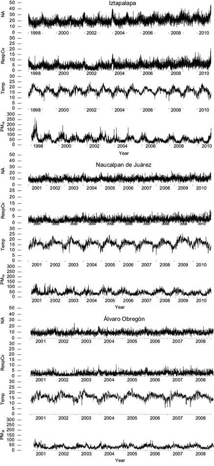
Fig. 1 Daily time series of non-accidental mortality (NA), cardiovascular and respiratory diseases (RespCV), temperature (Temp), and levels of particulate matter with an aerodynamic diameter less than 10 µm for Naucalpan de Juárez and Álvaro Obregón during the period 2001-2010, and for Iztapalapa during the period 1988-2010.
3. Model and estimation strategy
Murray and Nelson (2000) propose a state-space model that allows, through the observed mortality data, to estimate and study the dynamics of the at-risk population usually unobserved. Without a doubt, knowing the size and dynamics of the population at risk will increase our understanding of the relationship between pollution and individuals’ health of the at-risk population. Thus, one of our aims was to plot the at-risk population of these municipalities over time using their observed mortality data. Following Murray and Nelson (2000), we assumed that part of the population of these municipalities is at risk, subject to a risk rate that varies with atmospheric conditions including total suspended particles and temperature. New entrants will eventually replace the at-risk population that dies. This at-risk population, the new entrants, as well as the hazard rate are not noticed but can be estimated by applying the Kalman filter to the daily atmospheric conditions and mortality counts. By means of the Kalman filter, it is possible to estimate the hazard rate over time, its relationship to atmospheric variables, and the trajectory of the unobserved at-risk population. Murray and Nelson (2000) claim that it is also possible in the state-space framework, to address the following questions: What is the size of the population at risk? What is the life expectancy of individuals within that population? What is the effect of changes in air quality over that life expectancy?
Contrary to the Poisson regression model widely used in this kind of analysis (e.g., Peng and Dominici, 2008), in the case of the state-space model the effect of an at-risk factor such as PM10 on mortality is indirect. As shown in the following lines, it is proportional to the size of the at-risk population that is not observed. If the at-risk population has been reduced by recent mortality due to an increase in the hazard rate, then the effects of a new increment on the hazard rate will be mitigated, since the at-risk population is temporarily smaller. In fact, it is this reap effect which allows us to estimate the unobserved at-risk population by the Kalman filter. If a higher hazard rate persists, then the mortality count will fall back towards its previous level, since mortality is limited, in the long run, to the rate of new arrivals. However, the life expectancy of individuals in the at-risk population will fall, and this alternative approach offers estimations of this effect.
At the core of the Murray and Nelson (2000) model, there is an unobserved at-risk population from which all no-traumatic deaths are assumed to happen. This at-risk population is the group of individuals whose health is threatened due to various reasons, even in the absence of environmental hazards. The model assumes that the at-risk population decreases its size due to deaths and replenishes it with the arrival of new members. The model focuses on people whose health is frail and that eventually die. These authors define the at-risk population on a given day as its value on the previous day, plus new entrants, minus deaths. A first-order difference equation accounts for daily changes in the at-risk population in the following way:
where P t is the unobserved at-risk population, N t is the number of new arrivals, and D t is the observed number of deaths, all of them on day t. Each member of the at-risk population faces a probability of death that is a function of the environmental conditions, including ambient air quality. Daily deaths are represented by the following equation:
Environmental x t hazards are expressed in a hazard function γ'x t that models the amount of risk that is reduced or increased daily by environmental and seasonal factors. The hazard function is the daily probability of death, and we assume that it is a linear combination of atmospheric variables, including an intercept term. We do not know what the correct hazard function is, as it is in the Poisson regression model. To do this, an exploration is required about various hazard functions, which will be known as models. Deaths are also allowed to occur at random, as captured by the random error term .
As we mentioned above, both short- and long-term exposure to PM have been linked to adverse health effects, including the following: (i) increased number of hospital admissions and/or emergency department visits (Dockery and Pope, 1994; Rodopoulou et al., 2014); (ii) negative respiratory symptomatology (Pope et al., 1995; Wu et al., 2016), and (iii) increased aggravation of chronic diseases in cardiovascular and respiratory system (Schlesinger, 2007; Belen et al., 2014). Therefore, as in Murray and Nelson (2000), our baseline model uses the following hazard function:
In this model, γ 0 is the constant probability of death in the absence of environmental effects, and γ 1 is the marginal effect of PM10 on mortality.
On the other hand, temperature has been considered as a potential risk factor that could lead to a series of adverse health outcomes (Zhang et al., 2015; Chen et al., 2017) and as a control for the effect of seasonality variation in atmospheric conditions on the health status. Moreover, there is a U-shaped relationship between temperature and mortality, with mortality being lowest at moderate temperatures and highest at extremely low and high temperatures (Kan et al., 2003). Therefore, since the correct hazard function is unknown, this requires an exploration of various plausible hazard functions. As in Murray and Nelson (2000), we explored some hazard functions by including ambient temperature to control for seasonality, and since the mortality-temperature relationship is non-linear, we also investigated the quadratic and interactive function of temperature with PM, as shown below.
In the basic model of Murray and Nelson (2000), where the time series of mortality analyzed was stationary, new members of the at-risk population were assumed to enter randomly with a constant mean N equal to the mean daily deaths, plus Gaussian errors. Given the high variability in the population growth rate on most of the MAVM municipalities, the time series of mortality counts that we analyzed are of a non-stationary nature. Therefore, we departed from Murray and Nelson at this point, assuming that the new members of the at-risk population are included as follows7:
Since the at-risk population P t and the new entrants N t are unobserved, the parameter of this dynamic model cannot be estimated by means of conventional methods. However, the unobserved components can be estimated by using the state-space technique. Casting the model in this form, makes it possible to use the Kalman filter for parameter estimation. The representation considers Eq. (2) as a measurement equation, that is:
Then, we write Eqs. (1) and (4) as the following state equation:
If we assume that the error terms are normally distributed, then we can estimate the parameters of the model employing a maximum likelihood technique. For instance, the parameters estimate in the above system can be obtained by starting with an initial guess for the state vector and its covariance matrix. Given the initially estimated parameters, the Kalman filter recursively generates the prediction equation. Ultimately, the filter generates estimates of the unobserved components P̂ t and N̂ t , as well as γ̂, σ̂ e , and σ̂ η . To calculate the mean life expectancy of subjects in the at-risk population, the reciprocal of the estimated mean hazard rate is used; besides, the daily average at-risk population deaths are the ratio of the average mortality to the daily average at risk-population.
4. Empirical results
Using Kalman filters, we estimated the observation and state equation by maximum likelihood. Table II, table III, table IV, table V, table VI and VII report the estimates and asymptotic standard errors of the five baseline settings of the risk function including various combinations of PM10 and average temperature (Avtem), the square of temperature, and the multiplicative interaction of PM10 with Avtem. A constant term is included in each one of the risk functions. Model 1 uses only PM10. Model 2 adds Avtem to Model 1. Model 3 adds the square of Avtem allowing for hazard rate that increases at both extremes of temperature. Model 4 is included for comparison purposes and uses only the Avtem variable. Finally, Model 5 allows the effect of PM10 and Avtem, so they depend on the value of each other by adding the Avtem*PM10, an interaction variable. Estimates are produced using the Kalman smoother, which uses all information available in the sample, thus providing a better in-sample fit, as compared with the basic Kalman filter, which only uses information available at time t.
Table II Parameter estimates for Iztapalapa state-space models (standard errors in parentheses). Non-accidental mortality counts.
| Parameter | Model 1 | Model 2 | Model 3 | Model 4 | Model 5 |
| γ 0 | 0.0517673* (0.013920) | 0.0711946* (0.015207) | 0.0731026* (0.014924) | 0.0813666* (0.016433) | 0.0698405* (0.015839) |
| PM10 | 0.0000428* (0.000015) | 0.0000489* (0.000018) | 0.0000471* (0.000017) | 0.0000861 (0.000062) | |
| Avtem | 0.0006401** (0.000298) | 0.0000330 (0.001020) | 0.0001982 (0.001200) | -0.0000038 (0.000876) | |
| Avtem2 | 0.0000182 (0.000029) | 0.0000209 (0.000035) | 0.0000231 (0.000024) | ||
| PM10 *Avtem | -0.0000025 (0.000004) | ||||
| σ e | 0.2863* (0.0527) | 0.2585* (0.0354) | 0.2597* (0.0358) | 0.2583* (0.0301) | 0.2612* (0.0375) |
| σ η | 19.5635* (0.4636) | 19.0177* (0.4941) | 19.0651* (0.5205) | 18.9513* (0.4971) | 19.1061* (0.5242) |
| AVERISPO | 372 | 238 | 247 | 222 | 256 |
| MLE (days) | 15-19 | 10-12 | 10-13 | 10-12 | 11-13 |
| DAVERISPD | 5.3% | 8.4% | 8.0% | 9% | 7.8% |
| ln(L) | -14060.123 | -14055.217 | -14055.064 | -14059.057 | -14054.914 |
| Model selection test: likelihood ratio test | Model 5 vs. Model 4: 8.28** Model 5 vs. Model 1: 10.41** Model 5 vs. Model 3: 0.30 |
Avtem: average temperature; AVERISPO: average at risk-population; MLE: mean life expectancy; DAVERISPD: daily average at-risk population deaths.
Significant at *1, **5 and ***10%.
Table III Parameter estimates for Iztapalapa state-space models (standard errors in parentheses). Cardiovascular and respiratory mortality counts.
| Parameter | Model 1 | Model 2 | Model 3 | Model 4 | Model 5 |
| γ 0 | 0.0390000* (0.014156) | 0.0478247* (0.014572) | 0.0572752* (0.020528) | 0.052562* (0.020113) | 0.035773* (0.012902) |
| PM10 | 0.0000599* (0.000022) | 0.0000675** (0.000027) | 0.000056** (0.000026) | 0.0001829* (0.000067) | |
| Avtem | 0.0005804 (0.000373) | 0.001874*** (0.001052) | 0.002018 (0.001489) | -0.001452* (0.000524) | |
| Avtem2 | 0.000074*** (0.000042) | 0.000091 (0.000049) | 0.000069* (0.000026) | ||
| PM10 *Avtem | -0.000009 (0.000003) | ||||
| σ e | 0.0493* (0.0105) | 0.0464* (0.0075) | 0.0477* (0.0100) | 0.0465* (0.0075) | 0.05285** (0.0145) |
| σ η | 5.0243* (0.1235) | 4.9317* (0.1332) | 4.9768* (0.1364) | 4.9195* (0.1315) | 5.0583* (0.1191) |
| AVERISPO | 119 | 83 | 101 | 78 | 153 |
| MLE (days) | 18-25 | 12-18 | 6-13 | 12-16 | 25-34 |
| DAVERISPD | 5.8% | 8.4% | 6.9% | 8.9% | 4.5% |
| ln(L) | -10779.983 | -10777.679 | -10774.915 | -10779.770 | -10773.693 |
| Model selection test: likelihood ratio test | Model 5 vs. Model 4: 12.15* Model 5 vs. Model 1: 12.58* Model 5 vs. Model 3: 2.44 |
Avtem: average temperature; AVERISPO: average at risk-population; MLE: mean life expectancy; DAVERISPD: daily average at-risk population deaths.
Significant at *1, **5 and ***10%.
Table IV Parameter estimates for Naucalpan de Juárez state-space models (standard errors in parentheses). Non-accidental mortality counts.
| Parameter | Model 1 | Model 2 | Model 3 | Model 4 | Model 5 |
| γ 0 | 0.0344581** (0.013759) | 0.0424385* (0.000042) | 0.0475469* (0.015814) | 0.0497855* (0.014354) | 0.0400705* (0.014322) |
| PM10 | 0.000036*** (0.000019) | 0.0000422*** (0.000023) | 0.0000355*** (0.000021) | 0.0001398** (0.00008) | |
| Avtem | 0.0002985 (0.000213) | -0.0008906 (0.000771) | -0.0010178 (0.000732) | -0.0007899 (0.000843) | |
| Avtem2 | 0.0000375 (0.000026) | 0.0000437*** (0.000024) | 0.0000445* (0.000027) | ||
| PM10 *Avtem | 0.0000070* (0.000004) | ||||
| σ e | 0.0547* (0.0140) | 0.0525* (0.0111) | 0.0528* (0.0117) | 0.0536* (0.0118) | 0.0522* (0.01179) |
| σ η | 9.7460* (0.2626) | 9.6217* (0.2482) | 9.6520* (0.2537) | 9.6602* (0.2549) | 9.6887* (0.2589) |
| AVERISPO | 274 | 201 | 221 | 219 | 245 |
| MLE (days) | 25-32 | 19-22 | 19-23 | 19-23 | 21-27 |
| DAVERISPD | 3.6% | 4.9% | 4.5% | 4.5% | 4.0% |
| ln(L) | -9466.406 | -9464.690 | -9463.463 | -9465.930 | -9461.233 |
| Model selection test: likelihood ratio test | Model 5 vs. Model 4: 9.39* Model 5 vs. Model 1: 10.34** Model 5 vs. Model 3: 4.46** |
Avtem: average temperature; AVERISPO: average at risk-population; MLE: mean life expectancy; DAVERISPD: daily average at-risk population deaths.
Significant at *1, **5 and ***10%.
Table V Parameter estimates for Naucalpan de Juárez state-space models (standard errors in parentheses). Cardiovascular and respiratory mortality counts.
| Parameter | Model 1 | Model 2 | Model 3 | Model 4 | Model 5 |
| γ 0 | 0.0309206** (0.015591) | 0.0352771* (0.011758) | 0.0464546* (0.017443) | 0.0481114* (0.018152) | 0.0418381** (0.018547) |
| PM10 | 0.0000232** (0.000012) | 0.0000203*** (0.000015) | 0.0000158 (0.000015) | 0.0001117*** (0.000861) | |
| Avtem | 0.0003810*** (0.000279) | -0.0012113*** (0.000981) | -0.0012816 (0.001335) | -0.0011105 (0.001294) | |
| Avtem2 | 0.0000521*** (0.000030) | 0.0000557*** (0.000043) | 0.0000588 (0.000046) | ||
| PM10 *Avtem | -0.0000063 (0.000008) | ||||
| σ e | 0.0096* (0.0028) | 0.0093* (0.0020) | 0.0093* (0.0022) | 0.0092* (0.0021) | 0.0092* (0.0020) |
| σ η | 2.4501* (0.0687) | 2.4255* (.0525) | 2.4263* (0.0643) | 2.4250* (0.0643) | 2.4293* (0.0649) |
| AVERISPO | 79 | 59 | 60 | 59 | 63 |
| MLE (days) | 29-32 | 21-26 | 19-25 | 19-25 | 20-27 |
| DAVERISPD | 2.5% | 3.3% | 3.3% | 3.3% | 3.1% |
| ln(L) | -6928.885 | -6926.768 | -6925.972 | -6928.885 | -6925.684 |
| Model selection test: likelihood ratio test | Model 5 vs. Model 4: 6.40** Model 5 vs. Model 1: 6.56** Model 5 vs. Model 3: 0.57 |
Avtem: average temperature; AVERISPO: average at risk-population; MLE: mean life expectancy; DAVERISPD: daily average at-risk population deaths.
Significant at *1, **5 and ***10%.
Table VI Parameter estimates for Álvaro Obregón state-space models (standard errors in parentheses). Non-accidental mortality counts.
| Parameter | Model 1 | Model 2 | Model 3 | Model 4 | Model 5 |
| γ 0 | 0.0014023* (0.000359) | 0.0071729 (0.005121) | 0.0071047** (0.002813) | 0.0022783* (0.016433) | 0.0071041* (0.001885) |
| PM10 | 0.0000019** (0.0000008) | 0.0000163*** (0.000009) | 0.0000093* (0.000003) | 0.0000188* (0.000006) | |
| Avtem | -0.0001000** (0.000042) | -0.0002715** (0.000134) | -0.0000928* (0.000032) | -0.0002405* (0.000039) | |
| Avtem2 | 0.0000066 (0.000004) | 0.0000025** (0.000001) | 0.0000077* (0.000001) | ||
| PM10 *Avtem | 0.0000005* (0.0000002) | ||||
| σ e | 3.4531* (0.0624) | 0.0315* (0.0009) | 0.1124* (0.0026) | 2.1569* (0.0047) | 0.1089* (0.0634) |
| σ η | 9.1451* (0.2511) | 9.2280* (0.2687) | 9.15710* (0.2483) | 9.1676* (0.2369) | 9.1528* (0.2361) |
| AVERISPO | 6275 | 1501 | 1913 | 6371 | 1858 |
| MLE (days) | 625-714 | 128-185 | 166-227 | 55-714 | 158-217 |
| DAVERISPD | 0.14% | 0.59% | 0.47% | 0.14% | 0.48% |
| ln(L) | -7429.322 | -7423.335 | -7422.738 | -7425.923 | -7419.444 |
| Model selection test: likelihood ratio test | Model 5 vs. Model 4:12.95* Model 5 vs. Model 1: 19.75* Model 5 vs. Model 3: 6.58*** |
Avtem: average temperature; AVERISPO: average at risk-population; MLE: mean life expectancy; DAVERISPD: daily average at-risk population deaths.
Significant at *1, **5 and ***10%.
Table VII Parameter estimates for Álvaro Obregón state-space models (standard errors in parentheses). Cardiovascular-respiratory mortality counts.
| Parameter | Model 1 | Model 2 | Model 3 | Model 4 | Model 5 |
| γ 0 | 0.0022922* (0.000502) | 0.0019600* (0.000621) | 0.0066468* (0.002375) | 0.0124210* (0.003084) | 0.0087584* (0.003251) |
| PM10 | 0.0000065* (0.000001) | 0.0000061** (0.000002) | 0.0000123* (0.000004) | 0.0000105 (0.000022) | |
| Avtem | -0.0000413* (0.000013) | -0.0003802** (0.000174) | -0.0007212* (0.000238) | -0.0004931** (0.001294) | |
| Avtem2 | 0.0000093*** (0.000005) | 0.0000200* (0.000007) | 0.0000116 (0.000046) | ||
| PM10 *Avtem | 0.0000039*** (0.000001) | ||||
| σ e | 0.1590* (0.0040) | 0.1258* (0.0029) | 0.0293* (0.0004) | 0.0260* (0.0003) | 0.0183* (0.00007) |
| σ η | 2.5630* (0.0678) | 2.5735* (0.0643) | 2.5627* (0.0702) | 2.5521* (0.0671) | 2.5604* (0.0687) |
| AVERISPO | 1007 | 1681 | 739 | 419 | 565 |
| MLE (days) | 333-434 | 476-833 | 193-334 | 112-164 | 149-263 |
| DAVERISPD | 0.19% | 0.11% | 0.27% | 0.47% | 0.35% |
| ln(L) | -5563.340 | -5554.896 | -5553.908 | -5558.009 | -5552.023 |
| Model selection test: Likelihood ratio test | Model 5 vs. Model 11.9** Model 5 vs. Model 1: 22.63* Model 5 vs. Model 3: 3.77*** |
Avtem: average temperature; AVERISPO: average at risk-population; MLE: mean life expectancy; DAVERISPD: daily average at-risk population deaths.
Significant at *1, **5 and ***10%.
As for the analysis of each of the municipalities, Tables II and III show that when comparing the log-likelihood of Model 5 with that of Model 4, which does not include information about the levels of PM10, the likelihood ratio test suggests that, for non-accidental and cardiovascular-respiratory mortality causes, PM10 is highly significant in both populations. We can also observe that, when comparing Model 5 with Model 1, which does not include information about the level of Avtem, the likelihood ratio test suggests that Avtem is also highly significant in both populations. We also note that the interaction variable Avtem*PM10 is not significant in Model 5 when the log-likelihood is compared with that of Model 3; the likelihood ratio test suggests that Model 3 is preferable to Model 5. Thus, for Iztapalapa, we considered Model 3 as a reasonable baseline specification in both non-accidental and cardiovascular-respiratory deaths.
For non-accidental and cardiovascular-respiratory deaths, the hazard functions of Model 3 imply that both extremes of temperature are detrimental and that PM10 is also detrimental to the effect of rising temperature. At the average level of PM10 observed in the sample, the effect of an increase in temperature from the minimum (7 ºC) to the maximum (25 ºC) value is an increase in the hazard rate from 0.076 to 0.087 for non-accidental deaths, while for the cardiovascular-respiratory deaths the increment goes from 0.077 to 0.153. On the other hand, at the maximum temperature of 25 ºC, the effect of an increase of PM10 from the minimum (7 µg m-3) to the maximum (268 µg m-3) value observed in the sample is an increase in the hazard rate from 0.085 to 0.097 for non-accidental mortality, while for cardiovascular-respiratory deaths, the increase goes from 0.150 to 0.165. Consistent with previous studies (Samet et al., 2000a, b), the effects of an increase on the risk function are highest for cardiovascular and respiratory mortality than for non-accidental deaths.
Figures 2 and 3 plot the Kalman filter estimates of at-risk populations along with the estimated hazards rates in Model 3. The estimated at-risk population average is 247 for non-accidental deaths, but 144 for cardiovascular-respiratory deaths, and varies seasonally, with the daily number of deaths increasing to reach the highest level in winter. Since average mortality is 20 and seven deaths per day, this implies that about 8 and 6.9% of the at-risk population die on average per day due to non-accidental causes and cardiovascular-respiratory diseases, respectively. Hazard rates fluctuate seasonally as periods of high emission of PM10 and temperature extremes gather a severe harvest, followed by less lethal conditions. Historically, data suggest that the highest PM10 concentration occurs in the MAVM during late winter and early spring. We observed that, in the case of non-accidental deaths, the estimated at-risk population series moves higher with time, from an average of 216 at the beginning of the period to around 287 in the final years, while it moves from an average of 83 to around 123 in the same period for cardiovascular-respiratory deaths. There is a corresponding and offsetting decline in the hazard rate, moving downwards from an average of about 0.082 to 0.081 for non-accidental deaths, while it moves downwards from 0.113 to 0.112 for cardiovascular-respiratory deaths in the same period. This decline in hazard rates is driven by a reduction of about 65 to 47 µg m-3 in PM10 average emissions during the early and later years, respectively, and suggests that air control strategies implemented by the government since 1990 contributed to maintaining PM10 under a 24-h maximum limit and resulted in a decreasing trend during this period. The effect of this air control strategies on reducing PM10 emissions were also observed in the other two municipalities, as shown below.
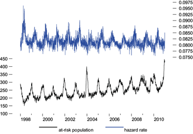
Fig. 2 Iztapalapa’s estimated at-risk population and hazard rate from Model 3. Non-accidental mortality counts.

Fig. 3 Iztapalapa’s estimated at-risk population and hazard rate from Model 3. Cardiovascular-respiratory mortality counts.
As pointed out by Murray and Nelson (2000), while an increase in risk factors cannot increase mortality, in the long run life expectancy is the inverse of the hazard rate, so hazard causing agents will shorten it. The hazard rates observed over the sample period go from 0.075 to 0.096 for non-accidental deaths, while they go from 0.075 to 0.157 for cardiovascular-respiratory deaths. Therefore, we have a life expectancy ranging from 10 to 13 days for the group of non-accidental death population, while life expectancy ranges from 6 to 13 days for the frail cardiovascular-respiratory death population.
Analogous to the Iztapalapa’s selection model, we have that, for Naucalpan de Juárez, the likelihood ratio test suggests that Model 5 is preferable for non-accidental deaths, while Model 3 is preferable for cardiovascular-respiratory deaths.
At the average level of PM10 observed in the sample, the effect of an increase in temperature from the minimum (5.44 ºC) to the maximum (25.82 ºC) value observed in the sample, is an increase in the Naucalpan de Juárez’s hazard rate from 0.045 to 0.063 for non-accidental deaths, and from 0.042 to 0.05 for cardiovascular-respiratory deaths. On the other hand, at the maximum temperature of 25.82 ºC, the effect of an increase in PM10 from the minimum (6.33 µg m-3) to the maximum (137 µg m-3) found in the sample is to raise the hazard rate from 0.051 to 0.093 for non-accidental deaths, while for cardiovascular-respiratory deaths, the increment goes from 0.050 to 0.052.
Figures 4 and 5 plot the Kalman filter estimates of the at-risk populations along with the estimated hazards rates in Models 5 and 3, respectively. The estimated at-risk population average is 245 for non-accidental deaths, while the average is 60 for cardiovascular-respiratory deaths, and, as in the case of Iztapalapa, it varies seasonally with the daily number of deaths, being the highest in winter. Since average mortality is 9.91 and 2.53 per day, this implies that about 4.0 and 3.3% of the at-risk population dies on average per day in the non-accidental and cardiovascular-respiratory populations, respectively. As in Iztapalapa, the hazard rates fluctuate seasonally as periods of high emissions of PM10 and of extreme temperature gather a grim harvest, followed by less lethal conditions. We observe that the estimated at-risk population series does move higher with time, from an average of 232, in the first years, to around 263 in the final years for non-accidental deaths, while it moves from an average of 60 to around 70 in the same period for cardiovascular-respiratory deaths. There is a corresponding and offsetting decline in the hazard rate, moving downwards from an average of about 0.040 to 0.039 for non-accidental deaths, while it moves downwards from 0.041 to 0.040 for cardiovascular-respiratory deaths in the same period. This decline in hazard rates is driven by a reduction of PM10 emissions of about 47.16 to 43.90 µg m-3 during the early and later years, respectively.
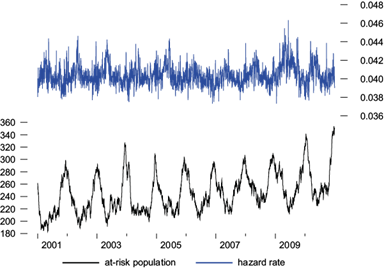
Fig. 4 Naucalpan de Juárez’ estimated at-risk population and hazard rate from Model 5. Non-accidental mortality counts.
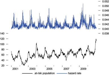
Fig. 5 Naucalpan de Juárez’ estimated at risk population and hazard rate from Model 3. Cardiovascular-respiratory mortality counts.
The hazard rates observed during the period considered in the sample go from 0.037 to 0.046, for non-accidental deaths, and from 0.039 to 0.051 for cardiovascular-respiratory deaths. Therefore, we have a life expectancy ranging from 21 to 27 days for non-accidental deaths, while life expectancy ranges from 19 to 25 day, for cardiovascular-respiratory deaths.
We observed that having a small at-risk population in Iztapalapa and Naucalpan de Juárez led to a clear mortality displacement, as the number of deaths fell below the average seasonal pattern after a high-risk event and did not return to the normal level until November. We also observed that the at-risk population was exhausted at the end of winter (the end of the risk period) and was mostly replenished by the middle of autumn (the end of the safest period).
Finally, in a way that is similar to the case of Iztapalapa and Naucalpan de Juárez, based on the likelihood ratio test results, Model 5 was regarded as a reasonable baseline specification in both non-accidental and cardiovascular-respiratory deaths for Álvaro Obregón.
As in the case of the previous two municipalities, we explored how PM10 and temperatures affect Álvaro Obregón’s hazard rate. Our results show that at the average level of PM10 observed in the sample, the effect of an increase in temperature from the minimum (5.80 ºC) to the maximum (23.94 ºC) value corresponds to an increase in the hazard rate from 0.0068 to 0.0069 for non-accidental deaths, while for cardiovascular-respiratory deaths the increase is from 0.0075 to 0.0076. On the other hand, at the maximum temperature level of 23.94 ºC, the effect of an increase of PM10 from the minimum (6.88 µg m-3) to the maximum (115.32 µg m-3) observed value in the sample consists in raising the hazard rate from 0.0059 to 0.0093 for non-accidental deaths, while for cardiovascular-respiratory deaths the increase is from 0.0043 to 0.0155.
Figures 6 and 7 plot the Kalman filter estimates of the at-risk populations along with the estimated hazards rates in Model 5. We observe a lower hazard rate with high variability, as compared with that of Iztapalapa, which is higher with low variability. A lower percentage of hazard lengthens life expectancy and allows individuals to remain longer in the at-risk population, thus making that population greater than the one in Iztapalapa and Naucalpan de Juárez. The estimated at-risk population average for non-accidental deceases is 1850, while the one for cardiovascular-respiratory deaths is 565 and varies seasonally; since average mortality is, respectively, 9.28 and 2.56 per day, this implies that, on average per day, about 0.48 and 0.35% of the at-risk population constitutes a case of either non-accidental or cardiovascular-respiratory death, respectively. The hazard rates fluctuate seasonally, according to the periods of high temperature. As in the other two cases, we noticed that the estimated at-risk population series does move higher with time, from an average of 1788 in the early years to around 1933 in the later years, for non-accidental deaths, and from an average of 473 to around 644 during the same period for cardiovascular-respiratory deaths. There is a corresponding and offsetting decline in the hazard rate, which moves downwards from an average of about 0.0050 in the early years to 0.0049 in the later years for non-accidental deaths, and from 0.0045 in the early years to 0.0044 in the later years for cardiovascular-respiratory deaths. This decline in the hazard rates is driven by a reduction of PM10 emissions of about 35.93 µg m-3 to 35.68 µg m-3 during the early and later years, respectively.
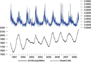
Fig. 6 Álvaro Obregón’s estimated at risk population and hazard rate from Model 5. Non-accidental mortality counts.
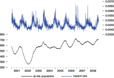
Fig. 7 Álvaro Obregón’s estimated at risk population and hazard rate from Model 5. Cardiovascular-respiratory mortality counts.
The hazard rates noticed over the sample period go from 0.0046 to 0.0063, in the case of non-accidental deaths, and from 0.0038 to 0.0067 in the case of cardiovascular-respiratory deaths. Therefore, life expectancy ranges from 158 to 217 days in the case of non-accidental deaths, and from 149 to 263 days in the case of cardiovascular-respiratory deaths.
The seasonal pattern in the at-risk population with a low hazard rate is interesting. We observed that, for a large at-risk population, the number of fatalities remained slightly below average for about two years. This longer-term impact on deaths is reflected in the mean life expectancy per high-risk event of 13 and 27 days for the small at-risk population of Iztapalapa and Naucalpan de Juárez, respectively, while the large at-risk population of Álvaro Obregón showed a mean life expectancy of 217 days.
5. Conclusions
The results of the analysis suggest that the main determinants of environmental health risk should be taken into consideration when assessing risk and vulnerability in urban populations. Our findings suggest that health risks related to air pollution are socioeconomically differentiated across the municipalities. Our estimates show evidence that various aspects of social inequality contribute to the greater burden of environmental hazard exposure and health risk for a municipality with low socioeconomic status. Social inequality, such as residential segregation, may affect the options of communities to address environmental and health problems. For example, poverty may affect the likelihood of having health insurance. Low education reduces knowledge and life skills that allow people to gain more ready access to information and resources to promote health (Link and Phelan, 1995). High population density may influence transportation demand, as expressed through average daily vehicle-kilometers traveled in private motor vehicles per capita; in turn, changes in transportation demand influence total vehicle emissions (vehicles for the transportation of passengers) to which population is exposed.
These socioeconomic disparities between municipalities partially explain why we observed a lower hazard rate in Álvaro Obregón, a wealthy area, as compared to the higher hazard rate observed in Iztapalapa, a poor area. In Álvaro Obregón-an area that showed a lower hazard rate-a higher life expectancy was observed, which allowsindividuals to stay longer in the at-risk population, thereby making that population larger than the at-risk population of Iztapalapa, whose inhabitants have a lower life expectancy. This is because the state-space model proposed applied the assumption that all fatalities must first be susceptible, so the smaller the at-risk population, the greater the individual probability of death. Therefore, the smaller the size of the population at risk, the sicker its average member will be, and hence the smaller the impact over long-term mortality. These findings are consistent with what would be normally predicted in texts about environmental justice.
As we already know, a proportion of these deaths occurs in susceptible people who would probably have died in the immediate future; however, a substantial number of them could have been prevented. Implementation of health policies should blunt some of the adverse impacts of air pollution on the pool of very frail people. We strongly believe that such health policies need to be addressed from the perspective of environmental justice.

