


 nueva página del texto (beta)
 Inglés (pdf)
 Artículo en XML
 Referencias del artículo
 Enviar artículo por email
 Citado por SciELO
  Similares en
SciELO
Similares en
SciELO 
 Permalink
1. Introduction
In the context of climate variability, the increasing attention to global warming emerging under the influence of anthropogenic activities has been associated with the consequences of its impacts, which ravage the natural structure of the ecosystem. The IPCC (2007) underlined that the proportional increase of greenhouse gases in the atmosphere would change the conventional climate structure in most parts of the world. It also reported (IPCC, 2013) that heavy rainfall events increased quantitatively towards the end of the 20th century. Hirabayashi and Kanae (2009) reported that more than 300 million people could be affected by even minor floods in 2060-2070. Considering only European countries, economic losses from floods in the next century are expected to rise from € 6.5 billions to € 18 billions (Cetin and Tezer, 2013). Concerning probable extreme precipitation in the future, Giorgi (2006) pointed out that the Mediterranean basin, in which Turkey is located, is among the most vulnerable regions that could be affected by climate change. Previous studies dealing with climate variability in Turkey indicate a remarkable alteration in the characteristics of precipitation (e.g., Turkes and Erlat, 2003; Turkes et al., 2009; Unal et al., 2012; Yurekli, 2015). Regarding precipitation, the most obvious impact of global warming on the world has appeared as floods and droughts, which are the most common and costly natural disasters. Among the probable natural catastrophes in Turkey, floods have caused most deaths and economic losses after earthquakes (Ozcan, 2008). During the period 1948-2015, flood events in Turkey affected 1 778 520 persons and resulted in 1350 fatalities. The economic loss associated with this natural disaster was estimated at USD 2.195 billion (Enginsu, 2015). Ozcan (2006) stated that floods commonly take place in the Black Sea, Marmara, and the Mediterranean regions in Turkey; even the Black Sea region has been exposed to flood events more frequently. Under this study, the Middle Black Sea region experienced 116 flood events in the period from 1956 to 2012, 80 of which occurred in the summer season. These floods caused 29 casualties, 4290 ha of cultivated land damaged, and 8051 homes and working places exposed to undesirable conditions. Seemingly, there has been a substantial increase in the number of floods during the last 15 years in the region (Enginsu, 2015).
Estimation of the magnitude and frequency of heavy rainfall causing floods is of great importance to understand their characteristic behaviour, in order to make decisions on water-related structures (Abolverdi and Khalili, 2010; Shahzadi et al., 2013). A frequent problem regarding the management and planning of water resources for reliable design is to estimate the probable magnitude of extreme rainfall or streamflow events due to the absence of adequate data concerning these events (Yurekli et al., 2009). In this sense, hydrologists have focused for several decades on the reliable analysis of available extreme data in their research (e.g. Kumar et al., 2003; Saf, 2009; Malekinezhad and Garizi, 2014; Ngongondo et al., 2011). The probabilistic characteristic of hydro-meteorologic variables is pivotal in designing water-related structures (Svensson and Rakhecha, 1998). Providing more reliable information about extreme events is crucially important to the management and planning of water resources within a regional context. The accuracy in the design of hydraulic structures is influenced mainly by the adopted frequency analysis approach and the quality and quantity of data used in the analysis.
The availability and quality of hydro-meteorological data is still a severe problem for hydrologists in many parts of the world (Easterling et al., 2000; Haddad et al., 2011; Hussain and Pasha, 2009). In cases where hydro-meteorological data is absent or insufficient in terms of quantity and quality, the regionalization method, referred to as regional frequency analysis, has been frequently used to assess extreme events (Lim and Lye, 2003; Zakaria et al., 2012). This approach consists of identifying the region, finding the sites compatible with each other in a region, applying an homogeneity test for the supposed region, and designating the regional statistical distribution (Sveinsson et al., 2002; Durrans and Kirkby, 2004). The method of L-moments has been widely used in the regionalization of hydrologic data, although there are different approaches for regionalization. Due to their several advantages over conventional moments (Sankarasubramanian and Srinivasan, 1999; Gubareva and Garstman, 2010), the procedure of L-moments has been adopted progressively in hydrologic studies by many researchers since the introduction of the approach (Abolverdi and Khalili, 2010; Modarres, 2010; Zakaria and Shabri, 2013; Anilan et al., 2015; Mosaffaie, 2015; Sarmadi and Shokoohi, 2015; Yin et al., 2015; Serra et al., 2016).
Even though several efforts have been made to perform regional frequency analysis (RFA) of heavy rainfalls on some parts of Turkey (e.g., Anli, 2009; Anli et al., 2009; Yurekli et al., 2009) during the last decades, no comprehensive studies in the Middle Black Sea Region (MBSR) in which destructive flood events have taken place in the last 15 years have been conducted in the context of RFA for extreme rainfalls. In the studies conducted by Yurekli et al. (2009) and Anli et al. (2009), the L-moments approach was applied to the annual maximum rainfall series of the Cekerek basin and Trabzon Province, respectively, whereas Anli (2009) performed this analysis on both the annual maximum and the partial-duration rainfall series for Ankara province. Seçkin and Topcu (2016) investigated the regional distribution behaviour of the annual maximum rainfalls belonging to 53 precipitation stations in Turkey using the L-moments method. It has been decided that the whole study area could be considered as a homogeneous region based on the heterogeneity test and the generalized logistic distribution has been determined as the most suitable distribution for the region. Ghiaei et al. (2018)) carried out a regionalization procedure based on L-moments on the annual maximum rainfall datasets with various durations from seven rainfall stations over the Eastern Black Sea Basin in Turkey. The generalized logistic (GLO) and generalized extreme value (GEV) distributions were determined for short-term (5 to 30 min) and long-term datasets (1 to 24 h) to estimate regional quantiles.
The specific objectives of the present study are: (a) to compute L-moments and its ratios; (b) to check the reliability of the data for the RFA; (c) to form groups of sites that satisfy the homogeneity condition; (d) to choose a regional frequency distribution; (e) to obtain L-moment ratio diagrams to select a candidate regional frequency distribution as an alternative way, and (f) to estimate quantiles based on the best fit distribution for the formed homogeneous region.
2. Materials and methods
2.1 Study area and data
Turkey consists of seven geographic regions, one of which is the Black Sea Region, which comprises three sub-sections, namely the Western Black Sea, Eastern Black Sea and Middle Black Sea. The MBSR lies between 39º-43º N and 34º-38º E (Fig. 1), with an elevation ranging from 2 m (Fatsa county) to 1287 m (Akkus county). The study area covers roughly 43 684 km2, approximately 5.6% of Turkey’s land area (Enginsu, 2015). The MBS has significant plains: Carşamba and Bafra in the coastal area and Niksar, Erbaa, Tasova and Suluova in the inland area. Kizilirmak and Yesilirmak rivers are the main water resources in the MBSR, which is geographically located in both river basins. The MBSR is under the influence of two different climate characteristics: a temperate oceanic climate affecting the coastal area and a continental climate reigning in the inland area. Precipitation amounts show a significant increase from the interior area towards the coastal zone. Annual rainfall varies from 600 to 800 mm in the coastal part, and decreases to 450 mm towards the inland. Heavy rainfall occurs in the coastal areas during autumn, whereas in inland areas it occurs during the spring (Sozer et al., 1990). Most floods in the period 2000-2012 were experienced across the coastal area (Enginsu, 2015). Kosarev et al. (2007) emphasized that large-scale atmospheric systems positioned over Eurasia and the North Atlantic have mainly become influential in the formation of the climate characteristics of the Black Sea.
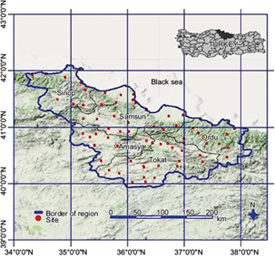
In the current study, daily rainfall data of 70 recording gauge stations compiled by the Turkish State Meteorological Service and General Directorate of State Hydraulic Works was used. Figure 1 shows the geographical location of the mentioned gauge stations in the study area and preliminary data associated with the sites are given in Table I. However, some recording gauge stations in the MBSR were discarded for a more reliable analysis due to very short record length and questionable data quality. Rainfall datasets belonging to the sites up to 2013 were used for regional frequency analysis in the study, but not every site had an observation length until 2013. There are two methods to choose the maximum rainfall series (Anli, 2009). The preferred method is based on selecting the maximum rainfall value of each year. In contrast, the other method (peak-over threshold, POT) is based on choosing all data greater than the considered threshold in a specific period. The overall approach, including selecting the annual maximum rainfall (hereafter referred to as AMR), has been preferred in the current study. The AMR value for daily rainfalls of the corresponding year for every gauge station was obtained.
Table I Geographic characteristics of the stations in the study area.
| Row | Sample size | Station name | Elevation (m) | Latitude (ºN) | Longitude (ºE) |
| 1 | 38 | Vezirkopru | 377 | 41.13 | 35.45 |
| 2 | 20 | Alicik | 700 | 40.80 | 35.31 |
| 3 | 79 | Amasya | 412 | 40.65 | 35.85 |
| 4 | 20 | Dogantepe | 520 | 40.60 | 35.61 |
| 5 | 31 | Aydinca | 675 | 40.56 | 36.15 |
| 6 | 25 | Goynucek | 530 | 40.40 | 35.53 |
| 7 | 39 | Gumushacikoy | 770 | 40.88 | 35.23 |
| 8 | 32 | Havza | 750 | 40.96 | 35.68 |
| 9 | 26 | Kavak | 741 | 41.09 | 36.05 |
| 10 | 47 | Ladik | 950 | 40.91 | 35.91 |
| 11 | 83 | Merzifon | 755 | 40.88 | 35.48 |
| 12 | 39 | Suluova | 490 | 40.83 | 35.65 |
| 13 | 24 | Bespinar | 721 | 41.00 | 35.00 |
| 14 | 53 | Mazlumoglu | 870 | 40.54 | 36.03 |
| 15 | 18 | Çakiralan | 950 | 41.00 | 35.00 |
| 16 | 81 | Tokat | 608 | 40.31 | 36.56 |
| 17 | 60 | Turhal | 500 | 40.40 | 36.10 |
| 18 | 53 | Zile | 700 | 40.30 | 35.90 |
| 19 | 50 | Almus | 830 | 40.25 | 36.56 |
| 20 | 47 | Artova | 1200 | 40.05 | 36.31 |
| 21 | 27 | Akkus | 1287 | 40.79 | 37.01 |
| 22 | 26 | Bereketli | 1125 | 40.51 | 37.30 |
| 23 | 27 | Camlibel | 1100 | 40.08 | 36.48 |
| 24 | 25 | Doganyurt | 530 | 40.68 | 36.71 |
| 25 | 62 | Niksar | 350 | 40.60 | 36.96 |
| 26 | 20 | Pazar | 540 | 40.28 | 36.30 |
| 27 | 30 | Resadiye | 450 | 40.16 | 37.38 |
| 28 | 38 | Resadiye / Zile | 790 | 40.13 | 35.42 |
| 29 | 31 | Hacipazari | 220 | 40.43 | 36.29 |
| 30 | 25 | Yolbasi | 1050 | 40.41 | 37.01 |
| 31 | 31 | Ekinli | 1070 | 40.02 | 36.20 |
| 32 | 30 | Sulusaray | 950 | 40.00 | 36.10 |
| 33 | 44 | Tasova | 200 | 40.76 | 36.33 |
| 34 | 47 | Erbaa | 230 | 40.70 | 36.60 |
| 35 | 12 | Camiçi | 1250 | 40.61 | 37.01 |
| 36 | 50 | Dokmetepe | 635 | 40.18 | 36.20 |
| 37 | 19 | Boztepe | 750 | 40.18 | 35.88 |
| 38 | 27 | Turkeli | 127 | 41.94 | 34.33 |
| 39 | 39 | Ayancik | 630 | 41.83 | 34.77 |
| 40 | 25 | Erfelek | 190 | 41.87 | 34.89 |
| 41 | 26 | Taflan | 150 | 41.00 | 36.00 |
| 42 | 24 | Duragan | 287 | 41.43 | 35.05 |
| 43 | 28 | Cerçiler | 700 | 41.00 | 35.00 |
| 44 | 26 | Dikmen | 385 | 41.66 | 35.27 |
| 45 | 21 | Kolay | 70 | 41.00 | 35.00 |
| 46 | 81 | Sinop | 32 | 42.02 | 35.15 |
| 47 | 50 | Engiz | 25 | 41.29 | 36.06 |
| 48 | 29 | Gerze | 86 | 41.81 | 35.17 |
| 49 | 65 | Bafra | 103 | 41.55 | 35.92 |
| 50 | 16 | Alacam | 7 | 41.63 | 35.63 |
| 51 | 48 | Boyabat | 350 | 41.46 | 34.78 |
| 52 | 54 | Unye | 16 | 41.14 | 37.29 |
| 53 | 26 | Fatsa | 2 | 41.04 | 37.48 |
| 54 | 24 | Hasanugurlu | 120 | 41.01 | 36.37 |
| 55 | 84 | Samsun | 15 | 41.28 | 36.33 |
| 56 | 56 | Çarşamba | 35 | 41.20 | 36.73 |
| 57 | 50 | Kizilot | 10 | 41.18 | 36.46 |
| 58 | 34 | Terme | 10 | 41.12 | 37.00 |
| 59 | 26 | Duzdag | 800 | 41.01 | 36.47 |
| 60 | 10 | Tekkiraz | 550 | 40.59 | 37.09 |
| 61 | 23 | Kumru | 735 | 40.85 | 37.24 |
| 62 | 49 | Gelemenagri | 4 | 41.40 | 35.55 |
| 63 | 33 | Golkoy | 1158 | 40.69 | 37.64 |
| 64 | 22 | Korgan | 725 | 40.00 | 37.00 |
| 65 | 24 | Topcam | 550 | 40.00 | 37.00 |
| 66 | 24 | Aybasti | 632 | 40.67 | 37.37 |
| 67 | 35 | Mesudiye | 1191 | 40.46 | 37.77 |
| 68 | 80 | Ordu | 5 | 40.98 | 37.88 |
| 69 | 13 | Perşembe | 190 | 40.98 | 37.70 |
| 70 | 20 | Ulubey | 190 | 40.87 | 37.75 |
2.2 L-moments approach
Recently, the L-moments method, popularized by Hosking (1990), has been adopted progressively in frequency analysis of hydro-meteorological variables due to its significant advantages over conventional product moments. Especially, they are relatively insensitive to the presence of outliers in a given series and they have no limits regarding sample sizes. Moreover, they define the structure of any statistical distribution more successfully and estimate the distribution parameters, particularly for hydro-meteorological data in circumstances where individual record lengths at gauging locations are relatively short, and compared with maximum likelihood estimates, they are commonly more tractable about computation. There is no need to transform the available data. On the other hand, compared to product moments, their estimators are almost unbiased, even in small samples, and are near normally distributed (Hosking, 1990; Park et al., 2001; Gubareva and Gartsman, 2010). The properties listed above make them preferable over product moments in frequency analysis of mostly roughly skewed hydro-meteorological data. L-moments are calculated based on probability-weighted moments (PWMs) characterized by Greenwood et al. (1979). A formal definition of the PWMs is provided here:
where F(x) is the cumulative distribution function (cdf) of a random variable X; X(F) is the inverse cfd related to X at F probability level, and r is the rth moment. In Hosking and Wallis (1997), L-moments are defined with regard to the PWMs as:
In Eq. (2), λ r + 1 represents the (r + 1)th L-moment.
For a given sample x 1 , x 2 …,x n , let x 1,n ≤ x 2,n ≤ … ≤ x n,n represent the order statistics of this series. Analogous to that of Eq. (2), the first four sample L-moments symbolized as l 1 , l 2 , l 3 , l 4 are:
In the Eq. (4,) b r (r = 0, 1 and 2…) is the sample probability weighted moments. Then, sample L-moments ratios, which are t(L-CV), t 3 (L-CS), and t 4 (L-CK) are defined as
L-CV, L-CS, and L-CK parameters are coefficients of variation, skewness and kurtosis, respectively.
2.3 Discordancy measure
Based on L-moments, a discordancy measure (D i ) is considered to screen for erroneous data and to check whether or not data are appropriate for achieving the RFA. A station is classified as discordant when its probabilistic behaviour is not like other stations of the region. D i is calculated based on a vector ui [ti, ti 3, ti 4]T, including sample L-moment ratios (L-CV, L-CS, and L-CK) of a site i (Hosking and Wallis, 1997). The discordancy measure is as follows:
N is the number of sites within the pooling group, and S is a matrix of cross-products. If any site i with Di > 3, the site is discordant (Hosking and Wallis, 1993; Rao and Hamed, 2000).
2.4 Regional homogeneity analysis
The heterogeneity (H) test proposed by Hosking and Wallis (1997) is based on the comparison of the between-site variation in the sample L-moments for a tentatively selected region, which has no discordant stations. Therefore, this test estimates the homogeneity degree in a group of sites. Three heterogeneity measures, named H 1 , H 2 , and H 3 are obtained by considering dispersion measures: L-CV, L-CS and L-CK. These H statistics depend on the 500 homogeneous regions simulated by population parameters equivalent to the regional average of L-moment ratios of the formed region sites (Hosking and Wallis, 1997; Tallaksen et al., 2004). Heterogeneity test statistics (H i , for i = 1,2 and 3) can be calculated by:
The values of V, V 2 and V 3 in Eq. (8) are estimated as:
where n i is the record length at site i, and t, t 3 , and t 4 are sample L-moments ratios; t R , t 3 R and t 4 R are the regional average of sample L-moments ratios, respectively; μ v and σ v are the mean and standard deviation of the V values estimated based on N sim , which represents the simulation data achieved by Monte Carlo simulation. The H-statistic value indicates that the formed region is acceptably homogeneous if H < 1, possibly heterogeneous if 1 ≤ H <2, and definitely heterogeneous if H ≥ 2.
2.5 Determination of the regional frequency distributions
After statistically confirming the group of sites as a homogeneous region, the best fit distribution to the homogeneous region is chosen by the goodness-of-fit-test (ZDIST), suggested by Hosking and Wallis (1997). This test is carried out based on the difference between the L-CK of the candidate distribution and the average L-CK of a homogeneous region under study. This test is given as:
where DIST represents a candidate probability distribution; t 4 DIST is the L-CK value dealing with the simulation for the corresponding distribution; t 4 R is the regional average of the at site L-CKs; β 4 is the bias associated with the regional average of the at site L-CKs, and σ 4 is the standard deviation belonging to the L-CK values based on the simulation data sets. The bias and standard deviation of regional average sample L-CK are calculated as follows:
where N sim is the number of the simulated regions with N sites, and t 4 [m] is the L-CK for the mth simulated region. To simulate 500 regions, close to the formed region, the four-parameter Kappa distribution is recommended to estimate β 4 and σ 4 . As highlighted by Hosking and Wallis (1997), the four-parameter Kappa distribution for simulation is preferred due to its capability for representing many distributions. According to their simulation analysis, the 500 value for N sim is generally sufficient. The parameters dealing with the Kappa distribution were estimated by using the regional average L-moment ratios. |ZDIST| ≤ 1.64 should be for a regional candidate distribution, but the numerically smallest distribution dealing with the |ZDIST| is taken as the best-fit distribution for the formed homogeneous region.
2.6 Prediction of regional quantiles
The well-known index-flood and index-storm approach in either streamflow or rainfall analysis, first introduced by Dalrymple (1960), has been widely used in regional quantile estimates dealing with environmental data. This procedure is based on the assumption that the sites forming a homogeneous region have an identical statistical distribution apart from index streamflow or rainfall value (a site-specific scaling factor) (Hosking and Wallis, 1997). Due to the use of rainfall data as material in our study, the work of Dalrymple (1960) will be hereafter referred to as the index-storm method. Mathematically, the quantile estimates at site i for a region with N sites are calculated by
where µ i is the index rainfall (a site-specific scaling factor) value for site i; F is the non-exceedance probability, and q is dimensionless distribution function (growth curve).
3. Results and discussion
Before applying the L-moments algorithm to the at-site data sets (AMR, otherwise known as block maxima) from rainfall gauging stations in the MBSR, low-order L-moments and its ratios for each site were calculated (Table II). As the first step for regionalization, the consistency among sites in the initially formed region is checked. The test on discordancy in the study was performed with a discordancy measure to assess whether or not there is inter-site consistency. In this sense, the prevalent attempt in RFA is that the whole study area (MBSR) is initially accepted as a homogeneous region. As seen from Table I, the topographic status of all rainfall gauging stations in the MBSR seems to be an obstacle for the evaluation of the entire area as an homogeneous region. Nevertheless, the above-described L-moments methodology was applied to at-site data sets under a presumption of a single homogeneous region. The results of the discordancy test dealing with a single homogeneous region covering 70 rainfall stations are given in Table II. According to the discordancy measure (D i ) results for each site, there is discordancy for six sites, namely Bereketli, Alacam, Fatsa, Hasanugurlu, Persembe, and Kumru. D values for these sites are bigger than the critical value (D critic = 3.0 for ≥ 15 sites in the region). The test statistic values of heterogeneity measures (H), namely H 1 , H 2 , and H 3 , were estimated as 5.84, 1.80, and 1.06, respectively. About these test values, the region covering 70 sites should be classified as definitely heterogeneous for H 1 , and possibly heterogeneous for H 2 and H 3 in terms of homogeneity, respectively. The L-moments procedure was reapplied to the region formed by the remaining sites after removing discordant sites to eliminate their undesirable impact on homogeneity. The second effort produced similar results. The heterogeneity test results for the region with 64 sites indicated that it was definitely heterogeneous for H 1 , possibly heterogeneous for H 2 , and acceptably homogeneous for H 3 . In comparison, four sites (Camici, Camlibel, Tekkiraz, and Gelemenagri) were discordant with the rest of the group. Hosking and Wallis (1997) highlight that the H 1 statistic has much better discriminative capability than H 2 and H 3 to distinguish homogeneity and heterogeneity. The values of H 2 and H 3 are rarely greater than two even in unpleasantly heterogeneous regions. Therefore, the H 1 statistic was considered when deciding on the homogeneity of a given region in the study. However, the results of the other two heterogeneity measures were also presented in this study.
Table II Summary statistics of the sites in the MBSR.
| Site | ℓ 1 | L-CV | L-CS | L-CK | D i |
| Vezirkopru | 39.25 | 0.1709 | 0.2717 | 0.2563 | 0.35 |
| Alicik | 29.70 | 0.1719 | 0.2076 | 0.1142 | 0.31 |
| Amasya | 32.56 | 0.1693 | 0.1833 | 0.1547 | 0.08 |
| Dogantepe | 30.49 | 0.2025 | 0.2805 | 0.2280 | 0.08 |
| Aydinca | 36.17 | 0.1484 | 0.1799 | 0.0483 | 1.20 |
| Goynucek | 35.60 | 0.1426 | 0.2880 | 0.1885 | 1.04 |
| Gumushacikoy | 32.50 | 0.1904 | 0.1704 | 0.1190 | 0.25 |
| Havza | 35.30 | 0.1480 | 0.1600 | 0.0660 | 0.79 |
| Kavak | 36.49 | 0.1122 | 0.1214 | 0.1394 | 0.90 |
| Ladik | 48.16 | 0.1871 | 0.3251 | 0.2470 | 0.38 |
| Merzifon | 27.91 | 0.1791 | 0.1854 | 0.1524 | 0.07 |
| Suluova | 30.70 | 0.1958 | 0.2827 | 0.1923 | 0.12 |
| Bespinar | 36.58 | 0.1671 | 0.2366 | 0.2694 | 0.54 |
| Mazlumoglu | 39.86 | 0.1767 | 0.1323 | 0.2394 | 1.18 |
| Çakiralan | 33.81 | 0.1210 | -0.0105 | 0.0316 | 1.67 |
| Tokat | 29.96 | 0.1688 | 0.1762 | 0.1973 | 0.21 |
| Turhal | 33.98 | 0.1583 | 0.2103 | 0.1948 | 0.17 |
| Zile | 32.50 | 0.1719 | 0.2478 | 0.2560 | 0.34 |
| Almus | 33.47 | 0.1839 | 0.2911 | 0.2275 | 0.18 |
| Artova | 29.06 | 0.1423 | 0.0981 | 0.1163 | 0.53 |
| Akkus | 54.11 | 0.2091 | 0.2524 | 0.1798 | 0.09 |
| Bereketli | 32.10 | 0.1615 | 0.2502 | 0.0022 | 3.15* |
| Camlibel | 24.97 | 0.1650 | 0.2056 | 0.3596 | 2.55 |
| Doganyurt | 39.24 | 0.1361 | 0.1183 | 0.0890 | 0.61 |
| Niksar | 33.34 | 0.1612 | 0.1835 | 0.1929 | 0.18 |
| Pazar | 28.53 | 0.1799 | 0.2904 | 0.3552 | 1.49 |
| Resadiye | 29.62 | 0.1435 | 0.1429 | 0.1200 | 0.37 |
| Resadiye / Zile | 31.92 | 0.1702 | 0.3559 | 0.2424 | 1.02 |
| Hacipazari | 35.10 | 0.2232 | 0.3072 | 0.2041 | 0.25 |
| Yolbasi | 51.78 | 0.1722 | 0.2045 | 0.0643 | 0.91 |
| Ekinli | 31.33 | 0.1351 | 0.1622 | 0.2643 | 1.31 |
| Sulusaray | 28.81 | 0.1554 | 0.2583 | 0.2469 | 0.50 |
| Tasova | 33.16 | 0.2313 | 0.4264 | 0.3307 | 1.13 |
| Erbaa | 33.98 | 0.1758 | 0.3045 | 0.2417 | 0.37 |
| Camiçi | 39.89 | 0.1589 | 0.4046 | 0.2496 | 2.21 |
| Dokmetepe | 31.65 | 0.1586 | 0.2352 | 0.2665 | 0.60 |
| Boztepe | 36.83 | 0.1717 | 0.0825 | -0.0204 | 1.81 |
| Turkeli | 52.47 | 0.2059 | 0.2802 | 0.2819 | 0.42 |
| Ayancik | 62.00 | 0.1551 | 0.0647 | 0.0992 | 0.80 |
| Erfelek | 56.10 | 0.1531 | 0.1409 | 0.1591 | 0.30 |
| Taflan | 55.28 | 0.1705 | 0.1746 | 0.1600 | 0.10 |
| Duragan | 30.91 | 0.1578 | 0.1009 | 0.0640 | 0.67 |
| Cerçiler | 37.55 | 0.1728 | 0.2864 | 0.2336 | 0.29 |
| Dikmen | 46.71 | 0.1116 | 0.2160 | 0.1412 | 1.44 |
| Kolay | 52.00 | 0.2110 | 0.2935 | 0.1709 | 0.29 |
| Sinop | 49.91 | 0.2530 | 0.3146 | 0.2368 | 0.66 |
| Engiz | 53.90 | 0.2489 | 0.3965 | 0.3085 | 0.91 |
| Gerze | 49.76 | 0.2007 | 0.2197 | 0.1213 | 0.30 |
| Bafra | 52.38 | 0.1848 | 0.1070 | 0.0892 | 0.67 |
| Alacam | 52.18 | 0.2593 | 0.0125 | 0.0729 | 5.20* |
| Boyabat | 36.59 | 0.2574 | 0.3815 | 0.1707 | 1.49 |
| Unye | 84.35 | 0.2660 | 0.3295 | 0.1624 | 1.30 |
| Fatsa | 98.11 | 0.3545 | 0.4520 | 0.2591 | 4.38* |
| Hasanugurlu | 66.47 | 0.3307 | 0.4253 | 0.2706 | 3.16* |
| Samsun | 55.14 | 0.2251 | 0.3381 | 0.2696 | 0.38 |
| Çarşamba | 63.13 | 0.1935 | 0.1424 | 0.1754 | 0.54 |
| Kizilot | 63.73 | 0.2364 | 0.3701 | 0.2949 | 0.65 |
| Terme | 65.61 | 0.2095 | 0.2596 | 0.2784 | 0.51 |
| Duzdag | 104.35 | 0.1910 | 0.1775 | 0.2020 | 0.31 |
| Tekkiraz | 71.91 | 0.2046 | 0.0681 | 0.2022 | 2.48 |
| Kumru | 53.80 | 0.2036 | 0.4561 | 0.4585 | 3.22* |
| Gelemenagri | 60.96 | 0.3152 | 0.4306 | 0.3296 | 2.67 |
| Golkoy | 57.67 | 0.1764 | 0.1424 | 0.0629 | 0.64 |
| Korgan | 46.83 | 0.1509 | 0.2263 | 0.2093 | 0.33 |
| Topcam | 42.10 | 0.1808 | 0.2835 | 0.1475 | 0.54 |
| Aybasti | 49.69 | 0.1673 | 0.1437 | 0.0464 | 0.84 |
| Mesudiye | 33.19 | 0.2080 | 0.3099 | 0.1551 | 0.57 |
| Ordu | 69.25 | 0.2002 | 0.3115 | 0.2341 | 0.19 |
| Perşembe | 75.51 | 0.1451 | -0.0601 | 0.1299 | 3.42* |
| Ulubey | 73.89 | 0.2566 | 0.2663 | 0.1145 | 1.39 |
ℓ 1: first sample L-moment (mean); D i : discordancy.
*Discordant site.
Based on the results of the first and second attempts on regionalization, the idea of evaluating the entire MBSR as a homogeneous region was disapproved. Similarly, the scatter diagrams of L-moment ratios (the L-CV vs. L-CS and L-CS vs. L-CK) also show that the initial proposal for regionalization is not suitable owing to quite high variability in L-moment ratios of the participating sites (Fig. 2). Then, the judgment from the assumption of one homogeneous region emphasizes that the MBSR should be divided into sub-regions until the homogeneity requirement is satisfied for each sub-region. For this purpose, the sub-regions were initially defined with the Ward’s clustering algorithm, which has been proposed by Hosking and Wallis (1997). The variables of elevation and latitude/longitude location associated with each site were used as a clustering variable in a preliminary determination of sub-regions. The results indicated that there were cases of two or more probable clusters. The inter-site consistency and homogeneity for each probable cluster (group) were checked by the discordancy measure and heterogeneity test. However, most sub-regions from the clustering method could not fulfil the requirement of inter-site consistency and homogeneity in the relevant region. Therefore, the at-site L-moment ratios were also considered together with the clustering approach in forming a homogeneous group. Moreover, the test results of groups ranging from two up to five were not satisfactory in terms of discordancy and homogeneity, except that of six groups. The most promising classification with a clustering approach was achieved by the Ward’s method with six clusters. Three of these sub-regions (regions 1, 2, and 5) covered 15, 22, and 11 sites, respectively (Table III). Figure 3 illustrates the final formation of sub-regions in the studied area. Inter-site consistency in the six sub-regions was proved with discordancy measure whose critical values (D critic = 3.0 for regions I and II, 1.92 for regions III and IV, 2.63 for region V, and 2.14 for region VI) were greater than the D value calculated for each site in the sub-regions. After reaching the judgment concerning the presence of inter-site consistency among sites forming each sub-region, the next step is to evaluate the homogeneity of a given sub-region in which the sites are assumed to have identical frequency distribution. In this study the homogeneity test was performed by applying heterogeneity measure (H 1 ) to each sub-region (Table IV). The H 2 and H 3 heterogeneity test results are also given in the Table IV. As can be seen from the table, all sub-regions have satisfied the homogeneity condition; in other words, six sub-regions were designated as acceptably homogeneous regarding the H 1 measure.

Fig. 2 Position of L-moment ratios with respect to each other for 70 sites. (a) L-CV vs. L-CS; (b) L-CS vs. L-CK.
Table III Homogeneous sub-regions (SR) and results of discordancy for the sites.
| SR-I | SR-II | SR-III | |||
| Site | D i | Site | D i | Site | D i |
| Vezirkopru | 0.64 | Tokat | 0.31 | Turkeli | 1.22 |
| Alicik | 0.38 | Turhal | 0.08 | Ayancik | 1.00 |
| Amasya | 0.06 | Zile | 0.13 | Erfelek | 0.72 |
| Dogantepe | 0.71 | Almus | 0.15 | Taflan | 0.10 |
| Aydinca | 1.21 | Artova | 0.82 | Duragan | 1.62 |
| Goynucek | 1.69 | Akkus | 1.22 | Cerciler | 0.68 |
| Gumushacikoy | 1.04 | Bereketli | 2.33 | Dikmen | 1.67 |
| Havza | 0.68 | Camlibel | 1.67 | ||
| Kavak | 1.77 | Doganyurt | 0.85 | ||
| Ladik | 0.77 | Niksar | 0.16 | ||
| Merzifon | 0.25 | Pazar | 0.87 | ||
| Suluova | 0.60 | Resadiye | 0.50 | ||
| Bespinar | 0.97 | Resadiye/Zile | 1.01 | ||
| Mazlumoglu | 2.02 | Hacipazari | 1.78 | ||
| Cakiralan | 2.21 | Yolbasi | 0.70 | ||
| Ekinli | 1.18 | ||||
| Sulusaray | 0.33 | ||||
| Tasova | 2.35 | ||||
| Erbaa | 0.22 | ||||
| Camici | 2.80 | ||||
| Dokmetepe | 0.30 | ||||
| Boztepe | 2.24 | ||||
| SR-IV | SR-V | SR-VI | |||
| Site | D i | Site | D i | Site | D i |
| Kolay | 0.28 | Unye | 1.59 | Golkoy | 0.55 |
| Sinop | 0.39 | Fatsa | 1.20 | Korgan | 0.92 |
| Engiz | 1.34 | Hasanugurlu | 0.73 | Topcam | 0.40 |
| Gerze | 0.44 | Samsun | 0.39 | Aybasti | 1.02 |
| Bafra | 1.01 | Carsamba | 0.68 | Mesudiye | 0.28 |
| Alacam | 1.85 | Kizilot | 0.29 | Ordu | 0.90 |
| Boyabat | 1.69 | Terme | 0.19 | Persembe | 2.11 |
| Duzdag | 0.51 | Ulubey | 1.81 | ||
| Tekkiraz | 2.18 | ||||
| Kumru | 2.36 | ||||
| Gelemagri | 0.88 | ||||
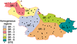
Table IV Heterogeneity test results for the six sub-regions.
| Heterogeneity measures | SR-I | SR-II | SR-III | SR-IV | SR-V | SR-VI |
| H1 | 0.17 | -0.46 | 0.70 | 0.69 | 0.94 | 0.57 |
| H2 | -0.73 | -0.99 | -0.04 | 2.52* | 0.22 | 0.78 |
| H3 | -0.47 | -0.48 | -0.41 | 2.06* | -0.34 | 0.49 |
*According to H 2 and H 3 , the sub- region is definitely heterogeneous.
The final step in RFA is to estimate an appropriate regional frequency distribution for the data of homogeneous sub-regions identified in the previous section. In our study, three-parameter distributions such as the Generalized Logistic (GLO), Generalized Extreme Values (GEV), Generalized Normal (GNO), Pearson Type III (PE3), and Generalized Pareto (GPA) distributions were considered as candidate distributions for sub-regions. Among them, those representing the regional data were determined according to the ZDIST statistic. It was decided that the distributions providing the basic assumption (|ZDIST| ≤ 1.64) dealing with this statistic could be used to make quantile estimates for the relevant region. The fitted regional distributions are given in Table V, where it can be seen that only the SR-II sub-region has a single regional distribution, while in the rest more regional distributions are selected for quantitative estimation. However, when many distributions were determined to be suitable for regional data in a specific region, the one with the smallest Z-statistic was selected as the most suitable. In this context, GEV for regions SR-I and SR-III, GLO for regions SR-II and SR-V were shosen as the most appropriate distributions. On the other hand, both GEV and GNO had the same and smallest Z-statistic value for SR-IV. The SR-VI region reached the smallest Z-statistic value in the GNO distribution. These results emphasize that GEV and GLO perform very well in fitting to the AMR data in the MBSR, so their test results are found to be acceptable in five sub-regions. The GNO distribution has the second-best performance after that of GEV and GLO due to its adequacy in four sub-regions. In comparison, PE3 is acceptable three sub-regions and GPA is not a candidate distribution in any of the six sub-regions. In many studies on frequency analysis of hydro-meteorological datasets (e.g., Coles, 2001; Katz et al., 2002; Ribatet et al. 2007; Aghakouchak and Nasrollahi, 2010; Obeysekera and Park, 2013; Li et al. 2015; Aziz et al., 2020) it is highlighted that AMR and POT data sequences are compatible with the GEV and GPA distributions, respectively.
Table V Test results based on goodness of fit ZDIST statistic for the six sub-regions.
| Homogeneous regions | Candidate distributions | ||||
| GEV | GLO | GNO | GPA | PE3 | |
| SR-I | -0.44 | 1.64 | -0.94 | -5.21 | -1.98 |
| SR-II | -2.02 | -0.15 | -2.73 | -6.51 | -4.04 |
| SR-III | -0.36 | 0.96 | -0.53 | -3.25 | -1.00 |
| SR-IV | 0.30 | 1.34 | -0.30 | -2.36 | -1.36 |
| SR-V | -1.58 | -0.86 | -2.28 | -3.64 | -3.48 |
| SR-VI | 0.72 | 1.84 | 0.25 | -2.00 | -0.59 |
Characters in bold show a suitable regional distribution.
Another attempt on distribution selection for a homogeneous region is a graphical approach (L-moment ratio diagram) which provides a quick visual assessment and compares the sample L-moment ratios with their theoretical counterpart (Peel et al., 2001). L-moment ratio diagrams (Fig. 4) drawn for each sub-region present similar results to the findings based on the ZDIST statistic. The points denoted by regional average values of L-CV and L-CS on the diagrams were acceptably close to the theoretical curves of distributions fitted to the data in Table V. The proximity to the curve of the candidate distributions included in the current study highlights a probable suitable regional distribution.
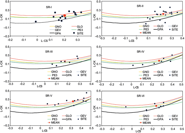
Fig. 4 L-moment ratio diagrams of L-CS vs. L-CK associated with SR-I, SR-II, SR-III, SR-IV, SR-V, SR-VI sub-rainfall homogeneous regions.
The estimation of regional rainfall amounts was accomplished by using the index-storm method given in Eq. (12). By taking the mean annual rainfall of the sub-region as index rainfall for that purpose, the regional rainfall amounts at return periods of 1, 2, 5, 10, 20, 50, and 100 years were obtained based on the corresponding values of growth factors (Table VI). As shown in Table VI, there is no significant difference among the regional AMR values estimated in the -regions where the multiple regional distributions are appropriate, except for the 1-yr return period. According to these results, the distributions found to be acceptable for the sub-regions can be used in the RFA. The choice should be the regional distribution with the minimum |ZDIST|, especially for the return periods that lead to differences between estimates.
Table VI Annual rainfall amounts estimated from suitable regional distributions.
| Region | Distribution | T (years) | 1 | 2 | 5 | 10 | 20 | 50 | 100 |
| F | 0.999 | 0.500 | 0.200 | 0.100 | 0.050 | 0.020 | 0.010 | ||
| SR-I | GEV | q(F) | 2.782 | 0.939 | 0.743 | 0.663 | 0.604 | 0.546 | 0.510 |
| Q(F) | 96.9 | 32.7 | 25.9 | 23.1 | 21.0 | 19.0 | 17.8 | ||
| GLO | q(F) | 3.336 | 0.944 | 0.753 | 0.663 | 0.593 | 0.518 | 0.471 | |
| Q(F) | 116.2 | 32.9 | 26.2 | 23.1 | 20.7 | 18.0 | 16.4 | ||
| GNO | q(F) | 2.709 | 0.939 | 0.740 | 0.661 | 0.606 | 0.554 | 0.523 | |
| Q(F) | 94.4 | 32.7 | 25.8 | 23.0 | 21.1 | 19.3 | 18.2 | ||
| SR-II | GLO | q(F) | 3.600 | 0.937 | 0.753 | 0.67 | 0.606 | 0.54 | 0.499 |
| Q(F) | 120.5 | 31.4 | 25.2 | 22.4 | 20.3 | 18.1 | 16.7 | ||
| SR-III | GEV | q(F) | 2.505 | 0.95 | 0.756 | 0.674 | 0.613 | 0.553 | 0.515 |
| Q(F) | 124.4 | 47.2 | 37.5 | 33.5 | 30.4 | 27.5 | 25.6 | ||
| GLO | q(F) | 3.011 | 0.954 | 0.766 | 0.675 | 0.602 | 0.523 | 0.472 | |
| Q(F) | 149.5 | 47.4 | 38.0 | 33.5 | 29.9 | 26.0 | 23.4 | ||
| GNO | q(F) | 2.487 | 0.95 | 0.753 | 0.672 | 0.614 | 0.558 | 0.524 | |
| Q(F) | 123.5 | 47.2 | 37.4 | 33.4 | 30.5 | 27.7 | 26.0 | ||
| PE3 | q(F) | 2.366 | 0.949 | 0.749 | 0.67 | 0.618 | 0.57 | 0.544 | |
| Q(F) | 117.5 | 47.1 | 37.2 | 33.3 | 30.7 | 28.3 | 27.0 | ||
| SR-IV | GEV | q(F) | 4.219 | 0.894 | 0.656 | 0.563 | 0.498 | 0.434 | 0.397 |
| Q(F) | 207.8 | 44.0 | 32.3 | 27.7 | 24.5 | 21.4 | 19.6 | ||
| GLO | q(F) | 5.015 | 0.901 | 0.664 | 0.562 | 0.485 | 0.407 | 0.361 | |
| Q(F) | 247.0 | 44.4 | 32.7 | 27.7 | 23.9 | 20.0 | 17.8 | ||
| GNO | q(F) | 3.872 | 0.891 | 0.65 | 0.562 | 0.504 | 0.452 | 0.423 | |
| Q(F) | 190.7 | 43.9 | 32.0 | 27.7 | 24.8 | 22.3 | 20.8 | ||
| PE3 | q(F) | 3.396 | 0.886 | 0.638 | 0.56 | 0.517 | 0.486 | 0.472 | |
| Q(F) | 167.3 | 43.6 | 31.4 | 27.6 | 25.5 | 23.9 | 23.2 | ||
| SR-V | GEV | q(F) | 5.304 | 0.869 | 0.639 | 0.554 | 0.496 | 0.44 | 0.407 |
| Q(F) | 364.2 | 59.7 | 43.9 | 38.0 | 34.1 | 30.2 | 28.0 | ||
| GLO | q(F) | 6.156 | 0.876 | 0.645 | 0.551 | 0.484 | 0.418 | 0.381 | |
| Q(F) | 422.8 | 60.2 | 44.3 | 37.8 | 33.2 | 28.7 | 26.2 | ||
| SR-VI | GEV | q(F) | 3.343 | 0.921 | 0.714 | 0.632 | 0.573 | 0.516 | 0.481 |
| Q(F) | 190.4 | 52.5 | 40.7 | 36.0 | 32.6 | 29.4 | 27.4 | ||
| GNO | q(F) | 3.156 | 0.919 | 0.71 | 0.631 | 0.577 | 0.528 | 0.5 | |
| Q(F) | 179.8 | 52.3 | 40.4 | 35.9 | 32.9 | 30.1 | 28.5 | ||
| PE3 | q(F) | 2.858 | 0.916 | 0.701 | 0.629 | 0.585 | 0.551 | 0.536 | |
| Q(F) | 162.8 | 52.2 | 39.9 | 35.8 | 33.3 | 31.4 | 30.5 |
Q(F): Regional rainfall amounts estimated by the index-storm method [μ i q(F)]; q(F): corresponding value of growth factors at different return periods based on the non-exceedance probability; μ i : index rainfall for site i (regional index rainfall is used for regional quantile estimation); F: probability; T: return period (1/F).
4. Conclusions
Floods are frequently experienced in the Black Sea region of Turkey. Numerous flood events have taken place in the study area (the MBSR) during the last 70 years. It is imperative to estimate possible future rainfall amounts to avoid floods and minimize their damages. The amounts in question are also predicted by frequency analysis. The current study was aimed to cope with regional frequency analysis of AMR data sequences by applying the L-moment regionalization procedure. The main conclusions are as follows:
After initially calculating low-order L-moments and their ratios for 70 sites, the existence of discordant stations to conclude whether or not there is inter-site consistency was checked with discordancy measure for the entire study area in terms of the possibility of forming a single homogeneous region. Six of the 70 sites had discordancy. Additionally, the results associated with the test statistics of three heterogeneity measures (H1, H2, and H3) pointed out that the whole MBSR should be classified as definitely heterogeneous for H1 and possibly heterogeneous for H2 and H3. These results prove that the region could not be considered as a single homogeneous region. When the MBSR was divided into six sub-regions, each sub-region satisfied the homogeneity test.
After weighing the inter-site consistency and homogeneity for six sub-regions, the candidate three-parameter distributions were selected based on the goodness of fit ZDIST statistic. The GEV and GLO distributions in five sub-regions, the GNO distribution in four sub-regions, and the PE3 distribution in three sub-regions were found to be acceptable for regional frequency distribution. In comparison, GPA was not a candidate distribution in any of the six sub-regions.
L-moment ratio diagrams, which are a graphical approach to the selection of regional frequency distribution, presented similar results to the findings from the ZDIST statistic.
The estimation of regional rainfall amounts was performed with the index-storm method. There was no significant difference among the regional AMR values estimated for the sub-regions where the multiple regional distributions are appropriate, except for the 1-yr return period. Nevertheless, the regional distribution with the minimum |ZDIST| should be considered in the regional rainfall quantile estimate, especially for the return periods that lead to differences between estimates.

