


 nueva página del texto (beta)
 Inglés (pdf)
 Artículo en XML
 Referencias del artículo
 Enviar artículo por email
 Citado por SciELO
  Similares en
SciELO
Similares en
SciELO 
 Permalink
1. Introduction
Land use and land cover change (LUCC) are among the major driving forces of regional and global climate change (Feddema et al., 2005). However, climatic effects of deforestation and agricultural development vary from one region to another, and studies clearly show that land use changes and land cover play an important biophysical and biochemical role in climate systems at local, regional, and even continental scales (Brovkin et al., 2013; Luyssaert et al., 2014; Mahmood et al., 2014). These also depend on seasonality and land-atmosphere interaction (Halder et al., 2016). Contemporaneous social and economic developments have intensified the impact of human activities on land surface temperature (LST). Urban development, due to the reduction in vegetation cover (Feng et al., 2012) and the increase in impervious materials such as concrete and asphalt (Connors et al., 2013; Hasanlou and Mostofi, 2015; Pal and Ziaul, 2017; Ziaul and Pal, 2018a), increases LST (Amiri et al., 2009). Other factors such as radiation conditions, heat conduction in the upper layer of the Earth’s surface, elevation from the surface of the Earth, relief, cloudiness, oceanic flows, and horizontal and vertical air flow are also important to determine LST. Therefore, intensity of land use can reflect the intensity of human activities, providing a basis to assess the relationship between land use change and environmental modifications.
LST is a major parameter in assessing the exchange of surface material, energy balance, and physical and chemical processes, and is now widely used in soil, hydrology, biology, and geochemistry studies (Tomlinson et al., 2011; Hao et al., 2016). Also, LST is an important factor in global studies, and heat stress is considered as a sign of climate change (Srivastava et al., 2009). Because of reflection from surface and roughness of different types of land uses, land use/land cover (LULC) changes are the main causes of LST variations (Hou et al., 2010). The soil LST is sensitive to vegetation cover and soil moisture, so it can be used to track land cover changes and land use, contributing to a better understanding of the desertification phenomena.
Fuzzy ARTMAP is an artificial neural network based on the adaptive resonance theory. The networks which work based on the adaptive resonance theory with supervised learning are known as ARTMAP (Carpenter et al., 1991). Each ARTMAP system consists of two modules (ARTa, ARTb) that create stable recognition classes in response to arbitrary sequences of input patterns. These two modules are connected to each other through an interface module called Fast Appearance-Based Mapping (Fab). The split-window algorithm requires only three parameters (emissivity, atmospheric emission, and average effective air temperature) to calculate LST. This algorithm was developed in 2001 to calculate the surface temperature by using the Landsat 5 Thematic Mapper (TM) sensor. With slight changes in the coefficients of the equations, it was then calibrated for other sensors (Rozenstein et al., 2014). This algorithm is based on mathematical analysis, and calculates LST by using ground data, a thermal infrared sensor (TIRS), land surface emissivity (LSE), and fractional vegetation cover (FVC), obtained from an operational land imager (OLI) (Latif, 2014).
LSTs can be estimated from infrared radiation, which is emitted from the surface, by the Stefan-Boltzmann inverse equation (Reutter et al., 1994). On the other hand, the Normalized Difference Vegetation Index (NDVI) is a good indicator of long-term changes in land cover and its status (Baihua and Isabela, 2015). It should be noted that an increase in temperature might raise the density of vegetation in areas with enough water resources (Xu et al., 2011). It has been demonstrated that there is a logical connection between NDVI and LST (Kustas et al., 2003; Weng et al., 2004; Agam et al., 2007; Inamdar et al., 2008; Wei et al., 2015). While temperature data, recorded by synoptic stations, are not useful for obtaining a good and wide spatial resolution, remote sensing (RS) images are a good source of information for the preparation of thermal maps, which is due to their extensive and continuous coverage, and timeliness (and the ability to obtain information in the reflection and thermal fields of electromagnetic waves) (Jiménez-Muñoz and Sobrino, 2010).
Due to the spatial correlation between data, conventional statistical methods are not suitable to analyze environmental data (Ripley, 1977). In this regard, various studies have been conducted to measure LST using RS technology (Herb et al., 2008; Feizizadeh et al., 2012. Qian et al., 2015; Isaya and Avdan, 2016; Fathizad et al., 2017; Deng et al., 2018; Li and Jiang, 2018; Ziaul and Pal, 2018 a, b; Tariq and Shu, 2020; Tariq et al., 2020).
Over the past decades, droughts, increased human intervention in soil and natural resources, degradation, rapid population growth, and increasing need for food and new energy resources have caused overexploitation of natural resources in Iran. Undoubtedly, the land use in the Ilam dam watershed has undergone some changes and can be a threat for the residents of the region. So, this study investigates the relationship between land use changes and LST over 28 years (1990-2018) using Landsat satellite imagery, and identifies land uses with the highest surface temperature in the study region. Due to the limited access to ground-based data, the satellite imagery has been used to study the temperature patterns.
2. Materials and methods
2.1. Materials
2.1.1 Study area
This research was conducted in the Ilam dam watershed in Iran (Fig. 1), with a total area of 47 652 ha, located at 46º 16’ 50’’-46º 38’ 56’’ E, 33º 23’ 24’’-33º 38’ 58’’ N, and 936-2584 masl. Figure 1 shows the location of the study area.
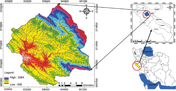
The study area forms a part of the folded Zagros zone. Zagros Mountains are a complex chain of ridges and mountains in SW Iran, extending NW-SE from the border areas of eastern Turkey and northern Iraq to the Strait of Hormuz. The Zagros range is about 1600 and 240 km long and wide, respectively. This mountain forms the extreme western boundary of the Iranian plateau and its foothills extend into adjacent countries. It divides the region between Iran’s dry inland plateau to the east and the fertile plains of Mesopotamia and the Persian Gulf lowlands to the west.
The main kind of vegetation in the Zagros forest habitat is oak trees. At altitudes above the forest border (about 2300 masl) there are dense grasslands and shrubs. In the west of Iran, especially in the Zagros region, oak is the most important and abundant tree species. The Zagros Mountains are the largest and most important habitat of various oak species in Iran, and therefore this region is of special importance.
2.1.2 Remote sensing data
In this research, Landsat Thematic Mapper (TM) imagery for 1990, 1995, 2000, 2005 and 2010 (pass/row: 167/37) with six spectral lines with a resolution of 30 m, and Landsat 8 (Operational Land Imager [OLI] Sensor) for 2015 and 2018 (pass/row: 167/37) bands 1 to 7 with a resolution of 30 m, band 8 with a resolution of 15 m and bands 9, 10 and 11 with a 30 m resolution were (Table I). Landsat images, published by the United States Geological Survey (USGS), were retrieved from the Earth Explorer website (http://earthexplorer.usgs.gov).
Table I Applied Landsat satellite imagery.
| Sensor | Data | Pass/row | Resolution (m) | Number of bands |
| MSS | 1985. 07. 22 | 167/37 | 60 | 4 |
| TM | 1990. 08. 29 | 167/37 | 30 | 7 |
| 1995. 08. 19 | 167/37 | 30 | 7 | |
| 2000. 08. 16 | 167/37 | 30 | 7 | |
| 2005. 10. 1 | 167/37 | 30 | 7 | |
| 2010. 07. 11 | 167/37 | 30 | 7 | |
| OLI | 2015. 08. 26 | 167/37 | 30 | 11 |
| 2018. 08. 18 | 167/37 | 30 | 11 |
MSS: Multispectral Scanner System; TM: Thematic Mapper; OLI: Operational Land Imager.
2.1.3 Software packages
ENVI 4.8, ArcGIS10.3 and Excel have been used in this study. The pre-processing works, including geometric and radiometric corrections, and post-processing tasks such as land use classification and LST layers have been extracted with the ENVI 4.8 software. ArcGIS 10.3 is used to provide the output of the maps and Excel is used to perform the statistical analysis.
2.2 Methodology
2.2.1 Pre-processing of images
The initial raw images of satellite data have incorrect geometry for reasons such as Earth orbits and changes in satellite elevation, in which case these images are not matched with the other satellite data. So, 35 ground control points from topographic maps were gathered for processing and interpreting multi-temporal satellite data. Further, the geometry of images was corrected in the ENVI 4.8 software environment by using the Global Positioning System (GPS).
Radiometric correction is necessary in remote sensing. Removing the undesirable effects of atmosphere is more important when the goal is comparing multi-temporal images (Chavez, 1988). In the present study, the Chavez method, which diminishes the value of dark object subtraction, is used for radiometric correction, and the value of dark object subtraction in the image is reduced to make the classification process highly accurate. For geometrical correction, topographic maps with a scale of 1.55000, prepared by the national geographical organization of Iran, were used. Images used in this research have been corrected by using ground control points and re-sampling equations. So, 45 ground control points with suitable distribution were used at the intersection of roads, waterways, etc., leading to a more accurate mathematical model. The average error obtained for the image sensor used was equal to 0.54 pixels, which is acceptable.
There are two types of radiometric corrections, absolute radiometric correction and relative radiometric correction. The absolute radiometric correction method requires data of atmospheric properties and sensor calibration. This type of correction is often very difficult, especially for older data (Du et al., 2002). In contrast, relative radiometric corrections are done with the aim of reducing the expected atmospheric variables, etc., between multi-time images. The dark-object subtraction technique is a simple relative radiometric correction method widely used in many cases (Chavez and MacKinnon, 1994). For radiometric correction, digital values are converted into spectral radiance in the first step by using the calibration coefficients of the sensor and the following equation:
where L is the spectral radiance (Wem-2 Ster-1 μm-1), DN the digital value of the pixel (0 to 255), and gain and offset are the calibration coefficients of the sensor. In the next step, according to Eq. (2), the amount of spectral radiance is converted into spectral reflectance (Richards, 2013; Lillesand et al., 2015):
where p is the spectral reflectance without units, from 0 to 1; L is the spectral radiance in the sensor; d 2 is the square of the distance between the Earth and the Sun based on astronomical units; ESUN is the height of the Sun, and SZ is the angle of the Sun when radiating while recording a satellite image.
By converting spectral radiance values to spectral reflectance, the effects of changes in the Sun light, season, latitude, and weather conditions on the images are eliminated. The outcome is relatively standard and can be used to directly compare the reflections of phenomena between different images and an image at different times. In this study, the method of reducing the darkness of the phenomenon, which is implemented in ENVI software, has been used for radiometric correction. This process is to reduce the effects of atmospheric diffusion on the image.
2.2.2 Post-processing of images
After geometric and radiometric corrections of the satellite image and cutting it in the study area, the land use map was extracted by using the fuzzy ARTMAP supervised classification method to six land use types of fair rangeland (26-50% of climax condition), poor rangeland (0-25% of climax condition), dense forest (canopy cover less than 25%), sparse forest (canopy cover more than 25%), agricultural land, and a water body. The main advantage of the fuzzy ARTMAP is that it requires lower training data for accuracy analysis compared with other methods. In addition, this method does not depend on the statistical distribution of data and does not require specific statistical variables. In order to verify the accuracy of the classification, a comparison was made with existing land use maps and field observations. In this way, the reference map or reality map from all parts of the study area was prepared by using other methods. A random sampling method was used to assess the accuracy of the obtained maps. Samples were recorded by using a GPS method in a number of polygons, by using a land use map and local views from the study area. In order to classify and separate the land uses of previous years from each other, the vegetation map of Ilam province (developed by the Forest, Range and Watersheds Management Organization of Iran [FRWO]) was used together with aerial photographs (1:20000) prepared by the National Cartographic Center of Iran (NCC).
Also, a split-window algorithm, which removes atmospheric effects, was developed and applied to estimate the emissivity and LST. In fact, LST is obtained by using the corrected thermal radiance. To calculate the corrected thermal radiance, it is necessary to determine the emissivity in the thermal bond.
2.2.3 Fuzzy ARTMAP classification method
The fuzzy ARTMAP method is a remote sensing classification based on neural network analysis and the Adaptive Resonance Theory (ART). The fuzzy ARTMAP supervised classification method consists of four layers: input layer (F1), category layer (F2), field layer, and output layer. The input layer represents the imported images, so there are some neurons to measure each criterion. The input layer for the infinity of the criterion is as follows:
In this method, the number of F2 layer neurons is automatically determined. The field layer and output layer are constructed with the ARTb model. Each of these two layers has m neurons. There is a one-to-one connection between these two layers.
2.2.4. Split-window algorithm for LST calculation
With this algorithm, LST is obtained by using corrected thermal radiance (Waters et al., 2002). To calculate the corrected thermal radiance, it is necessary to calculate the emissivity in the thermal bond. In fact, every land-related phenomenon is characterized by a specific emissivity, which was indicated by Snyder (1998). After detecting the minimum and maximum values, the NDVI is obtained; therefore, the average of soil and vegetation emissivity and the distribution of other areas can be calculated from Eq. (4).
Where εv and εs are the emissivity of areas with complete vegetation and areas with dry soil, respectively, and dε is the effect of surface distribution, which is calculated by using Eq. (5).
Where F is the form factor and its mean value is equal to 0.55, and Pv is the vegetation percentage, which is calculated by Eq. (6).
2.2.5. NDVI index
This index is one of the most practical indicators for vegetation studies. It has a simple computational process and has the best dynamic power compared to other indicators. This index is more sensitive to vegetation changes and less susceptible to atmospheric and soil effects, except in cases where vegetation is low. The NDVI index is derived from Eq. (7).
where NIR is the reflection in the near infrared band and RED is the reflection in the red band. From a theoretical point of view, the value of this index is in the range of ±1. The values of this indicator for dense vegetation cover tend to be +1. Clouds, snow and water are identified with negative values. Rocks and bare lands, with similar spectral responses in two bands, are seen at values close to zero. In this index, the common soil is equal to 1. Density of vegetation is determined by the distance between the indices of one pixel higher than the soil value (Allison, 1989).
2.2.6. Correction of LST
In this method, LST is obtained in ºK by using Eq. (8) (Artis and Carnahan, 1982).
Where LST is land surface temperature in ºK, λ is the wavelength of the desired band (11.5 μm) (Weng et al., 2004), ρ is the Boltzmann constant (Eq. 9), h is the Planck’s constant (6.626 × 10⁻³⁴), c is the speed of light (2.998 × 10⁸ m s-1), and T B is the brightness temperature in ºK obtained from Eq. (10).
K1 and K2 are correction coefficients with values of 666.09 and 1287.71, respectively (for Landsat images).
In ENVI, after obtaining the temperature of the black body and multiplying it by the coefficients of any phenomenon (emissivity), temperature can be calculated in ºC or ºK. It is also possible to calculate LST by using ENVI. Finally, the statistical parameters of each land use and LST for the years 1985, 1990, 1995, 2000, 2005, 2010, 2015 and 2018 are plotted on ArcGIS.
The final part of this procedure is the accuracy evaluation of the results. So, by using the ground control points, the correctness of calculations is evaluated by using the error matrix and statistical parameters of the total accuracy, kappa coefficient, and user’s and producer’s accuracy (Lu et al., 2004).
2.2.7. Accuracy assessment
Estimating accuracy is very important to understand the results and make decisions. The most common parameters for estimating accuracy are the overall accuracy, producer’s accuracy, user’s accuracy, and kappa coefficient (Lu et al., 2004). From a probability theory point of view, overall accuracy (Eq. 11) cannot be a good criterion for evaluating classification results; randomness may play a significant role in this index.
where OA is the overall accuracy, n is the number of experimental pixels, and P ii are the elements of the original diameter of the error matrix.
Due to the problems of overall accuracy, the kappa coefficient is often used in executive tasks where the comparison of classification accuracy is considered (Mesgari, 2002).
where P o stands for correctly observed and P c for expected agreement.
The producer’s accuracy is the probability that a pixel in the classification image will be placed on the ground in the same class, and the user’s accuracy is the probability that a specific class will be placed on the ground in the same class on the classified image (Eqs. 13 and 14)
where PA is the percentage accuracy of a class for producer’s accuracy, ta is the number of correct pixels classified as class a, ga is the number of class a pixels in ground reality, UA is the percentage accuracy of a class for user’s accuracy, and n 1 is the number of pixels in class a as a result of classification.
By cutting the classified maps with the ground reality map obtained from the field survey, an error matrix was formed to evaluate the accuracy of the classified maps, and based on that, the overall accuracy and the kappa coefficient were calculated.
3. Results
3.1. Land use map
In this research, a neural network fuzzy ARTMAP algorithm was used to determine and plot land use maps for 1990, 1995, 2000, 2005, 2010, 2015 and 2018 by using Landsat satellite images. Classes of Landsat images in the study area included rangeland, poor rangeland, dense forest, sparse forest, agricultural, and water body land use types. The land use map of the study area for 1990, 1995, 2000, 2005, 2010, 2015 and 2018 is shown in Figure 2.
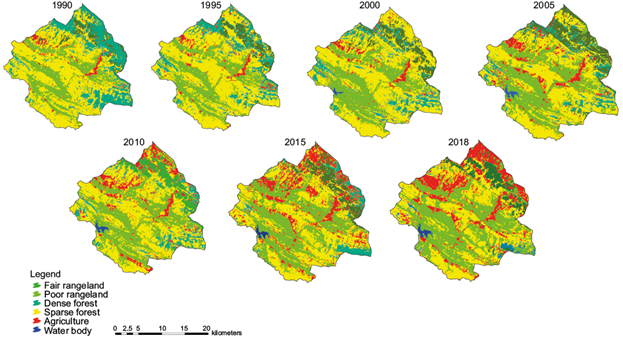
Fig. 2 Land use map of the study area based on the neural network fuzzy ARTMAP classification method for the years 1990, 1995, 2000, 2005, 2010, 2015 and 2018.
The results of the accuracy evaluation of the classified images are given in Table II, in which total, producer’s and user’s accuracy, as well as kappa coefficient, are also reported. High values of these coefficients indicate the acceptable accuracy for the land use identification by using RS data of Landsat images. It is observed that the classification accuracy for all the mentioned years is above 85%, which is an appropriate precision for classification of land uses.
Table II: Results of accuracy evaluation of the classified land use images for the period 1985 to 2018.
| Year/class | User’s accuracy | ||||||
| 1990 | 1995 | 2000 | 2005 | 2010 | 2015 | 2018 | |
| Fair rangeland | 0.67 | 0.73 | 0.78 | 0.75 | 0.74 | 0.81 | 0.85 |
| Poor rangeland | 0.95 | 0.95 | 0.95 | 0.94 | 0.94 | 0.99 | 0.97 |
| Dense forest | 0.8 | 0.94 | 0.96 | 0.92 | 0.88 | 0.95 | 1 |
| Sparse forest | 0.84 | 0.91 | 0.91 | 0.88 | 0.86 | 0.94 | 0.83 |
| Agricultural | 0.94 | 0.95 | 0.88 | 0.91 | 0.90 | 0.94 | 0.93 |
| Water body | - | - | 0.99 | 0.99 | 0.99 | 1 | 1 |
| Total accuracy (%) | 0.90 | 0.94 | 0.92 | 0.92 | 0.91 | 0.95 | 0.93 |
| Year/class | Producer’s accuracy | ||||||
| 1990 | 1995 | 2000 | 2005 | 2010 | 2015 | 2018 | |
| Fair rangeland | 0.81 | 0.99 | 0.93 | 0.96 | 0.94 | 0.98 | 0.99 |
| Poor rangeland | 0.96 | 0.93 | 0.96 | 0.94 | 0.94 | 0.97 | 0.94 |
| Dense forest | 0.85 | 0.88 | 0.88 | 0.85 | 0.84 | 0.93 | 0.69 |
| Sparse forest | 0.80 | 0.92 | 0.86 | 0.89 | 0.85 | 0.90 | 0.96 |
| Agricultural | 0.89 | 0.91 | 0.88 | 0.89 | 0.88 | 0.95 | 0.94 |
| Water body | - | - | 0.92 | 0.96 | 0.95 | 0.98 | 0.93 |
| Kappa coefficient (%) | 0.87 | 0.92 | 0.90 | 0.90 | 0.89 | 0.94 | 0.91 |
3.2. Land use changes
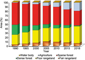
Results about changes in land use types of the study area during the investigated time periods are shown in Figure 3. They show that during the 28-year period (1990-2018), the area of agricultural land use has increased by 8650.6 ha (18.155%), highlighting an rise in population as well as in human pressure in the studied area. The most important land use change is related to dense and sparse forest land uses, with a decrease of 9867.14 and 8125.11 ha (20.07 and 17.04%), respectively. The study area has been conserved by governmental organizations in recent years. However, a decline in the extent of forest land use in the region is still seen. In a study that examined oak decline in the province of Ilam, results indicated a kind of ailment called charcoal disease (Biscogniauxia mediterranea) and borer beetles, which cause trees to die and fall. This disease has developed in recent years due to climatic conditions including rainfall reduction, drought and moisture stress which provide a suitable field for disease outbreaks (Mirabolfathi, 2013). Indeed, the rising demand for wood, timber, shelter and agricultural products has led to the destruction of natural land cover, especially forests that are becoming agricultural land at an alarming rate. The pressure from population growth has also led to uncontrolled alterations in exploitation, especially forestry in a wide area of the region. Hence, erosion and destruction of land are two of the most important current problems of this region. Negative effects of land use change in the study area include declining soil fertility, reduced vegetation and animal diversity, flood events, and increased landslide risk. The area of fair and poor rangeland land use types has increased by 1399.77 and 7652.16 ha (2.93 and 16.05%), which is due to the change of forest land to rangeland. Water bodies were not included in land use categories in 1985 and they were added in 2000. This land use is related to the Ilam dam, constructed in 2000 to supply drinking water.
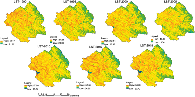
3.3. LST maps
According to LST maps (Fig. 4), the central and northwestern parts of the study area have a higher temperature because of agricultural activities, dense forest, and poor rangeland land use. LST maps (Fig. 4) show minimum LSTs of 21.27, 20.88, 25.37, 13.34, 28.85, 26.95 and 30.71 ºC and maximum of 54.18, 50.65, 52.85, 46.16, 57.51, 52.04 and 56.10 ºC for 1990, 1995, 2000, 2005, 2010, 2015 and 2018, respectively. In this study, the lowest temperature was due to dense forest land use in 1990, when the study area had a cool median temperature. However, overtime increases in the LST indicate climate change effects in the region, which could have devastating outcomes in the future. The maximum temperature drop of 2005 was caused by increased rainfall (above 600 mm) in the region, which led to an increase in vegetation cover in the study area.
3.4. Relationship between NDVI, LULC and LST
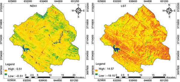
The LST is affected by different surface conditions, such that areas with vegetation accumulation tend to have lower LST than vegetation-free areas. By absorbing sunlight and transpiration of water through its leaves, vegetation creates a natural air-conditioning system. Changes from forest to rangeland and rain-fed farming land uses reduce the vegetation cover, remove the cooling system of natural surfaces and increase LST. Figure 5 shows the NDVI and LST differences between 1990 and 2018 in the study area. As it is obvious, wherever the vegetation has increased, LST has decreased and vice versa.
The results of the survey on average LST of the land uses in the study area for different years are shown in Table III. According to this table, the minimum temperature in 1990, 2010, and 2018 in dense forest was 3.5, 7.3 and 7.9 ºC, respectively, while the maximum surface temperature for sparse forest in 1990 and 2010 was 9.5, 11.8 ºC, and 10.9 ºC for dense forest in 2018. During most of the studied period, agricultural land had a lower average temperature than sparse forest and rangeland, which is mainly due to the high moisture content in agricultural land and the greater degree of evapotranspiration. Water bodies have the lowest average temperature due to the high-water heat capacity. Changes between 1990 and 2018 show that all land use types were subject to an increase in average temperature, which can be attributed to the increasing trend in temperature in the study area.
Table III: Temperature variations in different land uses (1990-2018).
| Class | 1990 | 1995 | ||||||
| Min. | Max. | Mean | Std. | Min. | Max. | Mean | Std. | |
| Fair rangeland | 33.17 | 51.11 | 42.93 | 3.34 | 27.99 | 43.09 | 35.65 | 2.70 |
| Poor rangeland | 28.80 | 54.18 | 44.02 | 3.10 | 22.70 | 50.65 | 40.68 | 2.97 |
| Dense forest | 21.27 | 51.46 | 38.25 | 4.15 | 20.88 | 46.54 | 35.61 | 4.29 |
| Sparse forest | 33.17 | 52.48 | 43.89 | 2.86 | 22.70 | 48.42 | 39.72 | 3.20 |
| Agriculture | 32.00 | 52.48 | 42.91 | 5.42 | 27.99 | 49.54 | 39.36 | 4.62 |
| Water body | - | - | - | - | - | - | - | - |
| Class | 2000 | 2005 | ||||||
| Min. | Max. | Mean | Std. | Min. | Max. | Mean | Std. | |
| Fair rangeland | 30.13 | 49.17 | 39.73 | 3.22 | 20.88 | 40.75 | 30.75 | 3.26 |
| Poor rangeland | 30.13 | 52.85 | 43.92 | 2.56 | 13.34 | 46.16 | 34.41 | 3.97 |
| Dense forest | 30.98 | 50.65 | 41.30 | 3.20 | 18.11 | 37.97 | 28.57 | 3.22 |
| Sparse forest | 25.37 | 51.02 | 42.01 | 3.81 | 19.51 | 42.71 | 32.72 | 3.75 |
| Agriculture | 31.40 | 50.28 | 42.92 | 3.65 | 22.25 | 44.25 | 35.52 | 3.80 |
| Water body | 27.55 | 40.36 | 32.09 | 3.00 | 23.15 | 31.40 | 24.85 | 1.76 |
| Class | 2010 | 2015 | ||||||
| Min. | Max. | Mean | Std. | Min. | Max. | Mean | Std. | |
| Fair rangeland | 35.95 | 49.91 | 43.49 | 2.39 | 33.66 | 49.56 | 41.54 | 2.72 |
| Poor rangeland | 29.28 | 57.15 | 48.13 | 3.39 | 28.66 | 52.04 | 44.11 | 2.71 |
| Dense forest | 30.55 | 57.51 | 44.39 | 4.60 | 26.95 | 50.23 | 37.31 | 4.25 |
| Sparse forest | 32.24 | 56.09 | 48.20 | 3.17 | 31.46 | 51.39 | 43.85 | 2.85 |
| Agriculture | 32.24 | 57.15 | 46.17 | 4.60 | 29.24 | 51.41 | 43.92 | 3.70 |
| Water body | 28.85 | 45.02 | 33.20 | 3.53 | 29.65 | 43.28 | 32.09 | 2.42 |
| Class | 2018 | |||||||
| Min. | Max. | Mean | Std. | |||||
| Fair rangeland | 34.83 | 51.12 | 43.20 | 2.77 | ||||
| Poor rangeland | 30.71 | 54.92 | 46.90 | 3.26 | ||||
| Dense forest | 33.82 | 56.10 | 44.75 | 4.43 | ||||
| Sparse forest | 37.71 | 54.57 | 47.87 | 2.25 | ||||
| Agriculture | 33.22 | 55.20 | 46.86 | 4.08 | ||||
| Water body | 31.17 | 45.71 | 33.60 | 2.49 | ||||
In order to study the effect of land use changes on surface temperature, an LST map for different time periods between 1990 and 2018 was prepared and compared to the land use change map for the same time period (Fig. 6). The results show that there was an increase in average LST in areas where land use change increased, indicating an intensification in heat-producing human-based activities, such as conversion of forest land use to agricultural use.
3.5. The nature of LST changes and land use
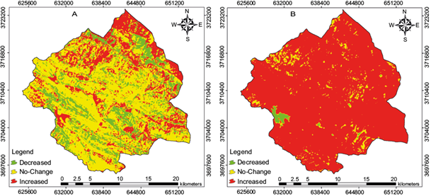
The crosstab method was used to investigate the land use and LST changes. In this method, classes of two classified maps are compared one by one. As a result, it is possible to determine the changes occurring in each class relative to the other. Figure 9 shows the crossed classified land use maps for 1990 and 2018, which exhibit the 1990 LULC variations compared to 2018. The difference in LST maps between 1990 and 2018 was used to examine LST changes (Fig. 5). The amount of various land use changes and the LST changes are shown in Figure 7 and Table IV. As Table IV shows, average temperature for all land use changes was positive and increasing, with the exception of dense forest, sparse forest and agricultural land, where LST dropped to -12.4 ºC.
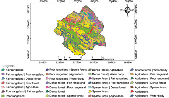
Fig. 7 Land use change map (1990 to 2018). In the map legend, each color indicates how the land use has changed over time. Some colors show two land uses, meaning that the area has changed from one land use to another. Some colors show only one land use, indicating no change in the land use.
Table IV: Results of land use and LST changes.
| LST (ºC) Class | Min. | Max. | Mean | Std. |
| Fair rangeland | Agriculture | -4.6 | 8.4 | 2.9 | 1.4 |
| Dense forest | Poor rangeland | -1.0 | 10.2 | 6.0 | 1.4 |
| Dense forest | Fair rangeland | -0.5 | 9.0 | 5.3 | 1.2 |
| Agriculture | -5.1 | 14.6 | 3.7 | 2.5 |
| Poor rangeland | Agriculture | -4.7 | 8.9 | 2.9 | 2.0 |
| Poor rangeland | Fair rangeland | 3.0 | 6.4 | 4.4 | 1.1 |
| Sparse forest | Agriculture | -4.7 | 9.5 | 3.3 | 1.6 |
| Dense forest | Agriculture | -3.3 | 9.4 | 4.2 | 1.7 |
| Poor rangeland | -10.6 | 9.5 | 4.1 | 1.6 |
| Sparse forest | Fair rangeland | -0.4 | 7.4 | 3.3 | 1.3 |
| Sparse forest | Poor rangeland | -10.2 | 9.9 | 4.9 | 1.5 |
| Fair rangeland | -1.4 | 7.7 | 3.9 | 1.1 |
| Dense forest | Sparse forest | -1.4 | 9.8 | 5.0 | 1.6 |
| Sparse forest | -2.8 | 9.9 | 4.0 | 1.4 |
| Fair rangeland | Sparse forest | -1.2 | 8.0 | 3.6 | 1.3 |
| Dense forest | -0.4 | 9.1 | 4.9 | 1.4 |
| Agriculture | Sparse forest | -0.8 | 10.4 | 4.6 | 2.4 |
| Poor rangeland | Sparse forest | 0.0 | 8.8 | 3.5 | 1.4 |
| Fair rangeland | Poor rangeland | -2.0 | 7.8 | 3.3 | 2.2 |
| Sparse forest | Dense forest | 0.9 | 7.5 | 4.0 | 1.2 |
| Fair rangeland | Dense forest | 1.7 | 6.1 | 4.3 | 0.8 |
| Agriculture | Poor rangeland | -9.0 | 14.1 | 4.9 | 2.8 |
| Agriculture | Fair rangeland | 4.3 | 7.5 | 5.8 | 0.8 |
| Agriculture | Dense forest | 2.7 | 5.2 | 4.4 | 1.0 |
| Poor rangeland | Water body | -19.2 | 0.2 | -10.8 | 3.5 |
| Sparse forest | Water body | -16.8 | 6.0 | -9.4 | 4.4 |
| Agriculture | Water body | -17.8 | -4.3 | -12.4 | 3.0 |
| Dense forest | Water body | -12.4 | -12.3 | -12.3 | 0.1 |
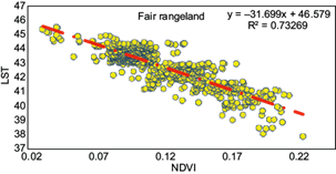
3.6. Relationship between LST and NDVI index
For better analysis of the relationship between LST and Land use, the correlation coefficients between LST and the NDVI index were calculated in 2018, based on randomized control points from each land use (Fig. 8). The highest correlation coefficient was obtained in dense forest and sparse forest land uses at 0.833 and 0.814, respectively. The lowest correlation coefficient (0.288) was related to water body land use, which confirms the lack of vegetation cover in this site compared to other land uses. Comparing the LST values of 2018 (Table III) and their correlation with the NDVI index (Fig. 8), it can be stated that in each land use where the average temperature is higher, the dependence between LST and NDVI is lower, indicating the low density of vegetation in these land uses. As shown in Figure 8, the correlation of the rangelands with the forest is lower, and their surface temperatures are higher than those of the forest.
3.7. Spatiotemporal distribution of LST
To study the spatial distribution of LST in the region, thermal images from different years were normalized by using the highest and lowest amount of surface temperature. Then, using average values and standard deviation, the normalized thermal images were classified into five temperature classes of low, medium, fairly high, high and very high limit. Figure 9 shows the thermal maps, and Figure 10 shows the area of temperature classes in the desired time periods. The results of the differences in areas between 1990 and 2018, show that the low, medium and fairly high limit classes decreased by 5, 15 and 20%, respectively, and the high and very high limit classes increased by 25 and 15%, respectively.
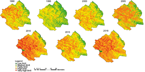
Fig. 9 LST classification maps using average values and standard deviation of thermal images (1990-2018) (in ºC).
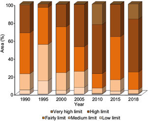
Due to the decrease in forest area and the increase in human-induced land uses, the area of lower temperature class has decreased, and the upper temperature class has experienced a notable increase during the time analyzed. The reduced area of dense forest and the increasing trend of agricultural and rangeland land uses indicate the replacement and conversion of the region’s natural coverage to lower value land uses. According to Figure 8, it can be said that the increase in LST is directly related to the increas in population density within the region and, consequently, the increas in agricultural area. The anticipated continuation of this trend provides grounds to expect a future (continued) rise in temperature (LST).
4. Discussion and conclusions
One of the important results of this research is the demonstration of the ability of fuzzy ARTMAP neural networks to classify land use types. Fuzzy classification includes methods that can provide results better suited to ground reality. In these methods, different values are calculated as the membership grade of each pixel based on land cover variation, while in definitive categorization methods each image pixel is attributed to only one class. The accuracy of the kappa coefficient for land use maps, derived from the satellite data classification by using the fuzzy ARTMAP classification for 1990, 1995, 2000, 2005, 2010, 2015, and 2018 is approximately equal to 87, 92, 90, 90, 89, 94 and 91%, respectively, which represents the high reliability of this algorithm in the classification of satellite data.
The results of the trend in land use change show that, in the period 1990-2018, most changes are related to agricultural lands and low-density (poor) rangeland, which have increased by 18.15 and 16.05%, respectively. On the other hand, land use types of dense forest and sparse forest have decreased by 20.70 and 17.04%, respectively, highlighting the destruction and change of natural and vegetated lands to cultivated lands. Another manmade land use that has many negative effects on nature is the construction of dams. From the time of construction of the Ilam dam (2005) until 2018, the water body behind the dam has increased by about 0.60%.
From LST maps, the range of surface temperature changed from 21.27 to 54.18 ºC in 1990 and from 30.07 to 56.09 ºC in 2018. Many scholars have focused on the relationship between the effects of land use change and LST. Results of Setturu et al. (2013) in the Uttara Kannada district (India), Pal and Ziaul (2017) in the English Bazar urban center of West Bengal (India), Fathizad et al. (2017) in southwest Iran, and Choudhury et al. (2019) in the Asansol-Durgapur Development show that land use changes are directly related to the increase in surface temperature. By examining the trend of temperature changes in the study area during the period 1990-2018, we observe an increase of 1.92 ºC, which is in line with the IPCC report of 2018.
The results of this study show that the LST has a high sensitivity to vegetation cover; land uses with higher vegetation density have lower surface temperatures. Hence, it can be used to detect changes in land use over time. With regard to the effects of land use changes, such as urbanization, establishment of communication roads, agricultural development and soil erosion in the study area, it can be predicted that surface temperature will increase in the future. It is evident that land use changes will result in changes in LST.
Further studies are required in this area under different seasons. Also, to achieve better results, particularly to more accurately estimate the LST, we suggest the use of image sensors with higher spatial resolution of the thermal bonding. In the future, more attention is needed to the modeling of land use changes, specifically by considering climate factors and detecting changes with different types of satellite images. This can reduce some degree of uncertainty in order to support management decisions. The results are potentially useful for various applications, including climatology, hydrology, ecology, geology, design and improvement of transport and agriculture networks.

