


 nueva página del texto (beta)
 Inglés (pdf)
 Artículo en XML
 Referencias del artículo
 Enviar artículo por email
 Citado por SciELO
  Similares en
SciELO
Similares en
SciELO 
 Permalink
1. Introduction
Friction velocity is one of the most important scaling parameters in atmospheric sciences and oceanography (Garrat, 1977; Stapleton and Huntley, 1995). Most processes and relationships in the low atmosphere involve the friction velocity, such as turbulent exchange of mass and energy at the surface and relationships based on the Monin-Obukhov Similarity Theory (Monin and Obukhov, 1954; Wyngaard et al., 1977) and on the surface renewal theory (Brutsaert, 1982; Stull, 1988; Castellví, 2018; Castellví et al., 2020). The friction velocity, u*, is defined as (Stull, 1988):
where u, v, and w are the x, y, and z components of the velocity vector; u’, v’ and w’ are the velocity fluctuations with respect to the mean velocity components U, V, and W (i.e., u’ = u - U). The overbar refers to time averaging. There are many different definitions of the friction or shear velocity (Weber, 1999) and the selection depends primarily on the particular application. Eq. (1) is related to the length of the Reynolds Stress vector when u is aligned with the mean velocity, hence this definition is independent of the chosen frame of reference and will be used in this report.
There are a variety of techniques to estimate u * (Champagne et al., 1977; Nieuwstadt, 1978; Durand et al., 1991; Bauer et al., 1992; Inoue et al., 2011; Newman and Klein, 2014). For instance, the eddy covariance (EC) method uses high frequency direct measurement of velocity fluctuations in the surface layer to obtain the friction velocity from Eq. (1) (Burba, 2013). The measurement can be made using hot wire, sonic or other type of anemometer, as long as (a) the three components of the velocity are measured, and (b) the acquisition frequency is large enough to capture the rapid turbulent fluctuations; note that the averaging period must not be too long in order to avoid contamination from slow non-turbulent signals or trends (usually between 30 and 60 min).
Sonic anemometers are convenient because they do not have moving parts (the measurement is based on the speed of sound). Two dimensional (2D) sonic anemometers are much more robust and affordable than triaxial sonic anemometers. Unfortunately, 2D sonic anemometers cannot be used to directly determine the friction velocity (Eq. 1) because the vertical wind component is not measured; however, an estimate of friction velocity could be obtained from the logarithmic wind profile (Echols and Wagner 1972; Bauer et al., 1992; Bergeron and Abrahams, 1992; Sozzi et al., 1998), but this method requires deployment of 2D anemometers at several heights. In this investigation, a method to estimate friction velocity from a single 2D anemometer is proposed and tested against field measurements.
2. Method
On the basis that the turbulent standard deviation of the horizontal wind speed does not follow similarity and it is well correlated with the friction velocity and the horizontal mean wind speed (Dyer, 1974; Panofsky et al., 1977; Sorbjan, 1987; Stull, 1988; Graefe, 2004; Banerjee et al., 2015), here a semi-empirical relationship is proposed to estimate the friction velocity using a 2D sonic anemometer capable to record (in a half-hourly basis) accurate values of the turbulent standard deviation of the horizontal wind speed and the mean wind speed as follows:
where a and b are coefficients that must be calibrated against the friction velocity determined using a triaxial sonic anemometer. Once a and b are known, the friction velocity from 2D measurements (u *2D ) can be estimated from Eqs. (2) and (3). Here the velocity vector was rotated in the mean wind direction (i.e., the cross-wind component), thus I is related to the turbulent intensity (Stapleton and Huntley, 1995; Pope et al., 2006; Yahaya and Frangi, 2009). Notice that Eq. (2) can be interpreted as a relationship between a drag coefficient and the turbulence intensity (it can be rewritten as C D ~ I 4b ), with the inconvenience that the measurements can be done at different heights above ground (see Table I), so it would not be a “standard” drag coefficient, but a local one (Mahrt et al., 2001).
Table I Characteristics of the experimental sites.
| Sisal meteorological mast (S1) | El Palmar (S2) | Estero el Soldado (S3) | Navopatia (S4) | Cape Tribulation (S5) | Gingin (S6) | |
| Latitude (˚) | 21.1647 | 21.0293 | 27.95 | 26.3999 | -16.1032 | -31.3763 |
| Longitude (˚) | -89.9533 | -90.0637 | -110.97 | -109.2397 | 145.4469 | 115.7138 |
| Type of terrain | Complex, no orography. 100 m from the coastline. Barrier island close to a town | Homogeneous. Tropical dry seasonal forest | Open water, coastal lagoon. Type: Arheic | Flat, homogeneous mangrove close to an estuarine lagoon | Tropical rainforest | Coastal plain woodland on SW Australia |
| Time-series dates | 2010/Jul/29- 2012/May/23 | 2018/Mar/15-2019/Aug/21 | 2019/Jan/01- 2019/Dec/31 | 2018/Jan/01- 2018/Dec/31 | 2011/Jan/01- 2011/Dec/31 | 2019/Jan/01- 2019/Dec/31 |
| Canopy height (m) | Variable | 11 | 0.1 | 5.0 | 23 | 6.8 |
| Roughness length z0 (m) | Direction-dependent (1 -6 to 1.5 -2 × 10⁻²) | 0.15 | 0.015 | 0.50 | 0.1 to 1 | 0.5 |
| Mean wind speed (m s-1) | 5.77 | 3.2 | 2.5 | 2.42 | 1.5 | 3 |
| Dominant wind direction | ESE | ESE | WSW | WSE | SE | SSW and SE |
| Sensor height to the ground (m) | 12.5 | 21.8 | 1.8 | 6.5 | 45 | 45 |
| Data set size (number of records) | 12 777 | 16 813 | 5962 | 13 253 | 16 849 | 14 819 |
3. Materials and field data
The proposed semi-empirical relationship (Eqs. 2 and 3) was calibrated at six sites with contrasting wind regimes. Table I shows the site locations and experiment characteristics (such as height above ground of the instruments, canopy height, measurement dates, number of records and mean wind speed). Figure 1 shows the map location (upper panel) and the wind roses for each location (lower panel). Note that a different color scale is used in S1 (wind rose) due to its high wind speed average. The site names (and acronyms in parenthesis) are also shown. They are grouped according to their geographical situation in: (1) Gulf of Mexico data sets, (2) Gulf of California data sets, and (3) Australia data sets.

Fig. 1 (a) Location of sites S1, S2, S3, and S4 in Mexico. In the Gulf of California, the site Estero el Soldado (EES, S3-triangle) and Navopatia (S4, dark diamond). To the SE, on the Yucatan Peninsula, El Palmar (S2, green triangle) and Sisal (S1, pentagon). (b) Location of sites S5 and S6 in Australia. In north Queensland, Cape Tribulation (S5, dark green diamond). To the SW, in Western Australia, represented by a green diamond, Gingin (S6). The lower panel shows the wind roses (wind speed in m s-1) for the six experimental sites, together with their respective notation.
EC experiments must be carefully assessed with statistical data quality tests (Foken and Wichura, 1996; Aubinet et al., 1999). Although most experiments carry out similar pre-processing (peak removal, detrending, gap filling), data quality control is always site-specific. There exist many quality control methods and indexes. Either method can be used with similar results, and stationarity tests are common due to its ease of implementation and interpretation. The method used for each experiment can be consulted in the next section (and references therein). This is important in this context because one cannot use the vertical component of the wind when using a 2D anemometer. However, one can construct stationarity or ogive tests with the horizontal components using the same principles (with the obvious exception of turbulence tests).
All bad data were previously eliminated by the site-specific quality control schemes. We had access to post-processed data using the EC technique (additionally we had raw data from S1 and S2). All sites used a half-hour averaging period. Another aspect of data processing that has to be brought to mind is wind velocity rotation; the post-processed data was already doubly (or triply) rotated, and a 2D measurement can only be rotated in one axis. This subject will be discussed in the last section, where a comparison with single vs. double (and triple) rotation is carried out to assess this issue quantitatively.
3.1 Gulf of Mexico datasets
The first and second experiments are Sisal (S1) and El Palmar (S2), respectively. They are shown in Figure 1a, both located at the NW of the Yucatan Peninsula in Mexico. S1 is situated at the beach (100 m to the shoreline), to the west end of the town of Sisal; a 50-m height mast equipped with five sonic anemometers at 3, 6, 12.5, 25 and 51 m from the ground was used to acquire wind data between August 2010 and September 2013. Two anemometers (12.5 and 51 m) were 3D (Thies 3.383x) and the rest were 2D (Thies 4.382x). This site is characterized by a bimodal wind speed U regime due to sea breeze (Figueroa-Espinoza et al., 2014). Dominant winds are ESE (seaward) and the average wind speed is 5.77 m s-1 at z = 12.5 m. Even though the terrain is flat, it is non-homogeneous because of the internal boundary layers caused by roughness effects on winds coming from different directions (Figueroa-Espinoza and Salles, 2014; Figueroa-Espinoza et al., 2014). Data pre-conditioning included a triple rotation for 3D anemometers, and single rotation for 2D (Wilczak et al., 2001). Data from a 3D anemometer at height z = 12.5 will be used unless specified otherwise. The second site is located 14 km south (inland) of Sisal, in a state reserve called El Palmar (S2 in what follows), a tropical-dry seasonal forest (Fig. 1c; see also Uuh-Sonda et al., 2018, 2021) in flat and homogeneous terrain whose average canopy height ranges from 8 to 12 m. In this site an EC tower is equipped with a WindMaster 3D anemometer at height z = 21.8 m. Data was post-treated with the EC technique, following Aubinet et al. (1999). A double rotation of the velocity vector was applied for all sites that adhere to this methodology (i.e., S2, S3 and S4) (Delgado et al. 2018; Balbuena et al., 2019; Uuh-Sonda et al., 2021). Prevailing wind directions are EES (Fig. 1d) and, despite being in the range of sea breeze influence (Taylor-Espinosa, 2009; Garza-Pérez and Ize-Lema, 2017), Uat S2 (~3.2 m s-1) < Uat S1 (5.8 m s-1). S1 data is freely available to the public (Figueroa-Espinoza and Salles, 2020), as well as S2 (Uuh-Sonda et al., 2020).
3.2 Gulf of California datasets
The two coastal sites from the Gulf of California used for this study were (Fig. 1a): Estero el Soldado (S3) and Navopatia (S4). S3 is located in a tidal coastal lagoon in the central region of the Gulf of California (Fig. 1e; Benítez-Valenzuela and Sánchez-Mejía, 2020). S3 has EC instruments including a WindMaster 2329-701-01 3D sonic anemometer deployed on a small floating platform (2 × 2 m) located at the inlet of the lagoon at 1.8 masl (Barreras-Apodaca and Sánchez-Mejía, 2018). Prevailing winds at S3 are WSW (landward; Fig. 1S3), with U = 2.5 m s-1. EC data for S3 is available at the public repository described in Benítez-Valenzuela et al. (2020). S4 is located within an estuarine system along the northern Mexican Pacific coast (Fig. 1a). It has an EC tower with instruments, including a Windmaster Pro 3D sonic anemometer, sitting 1.5 m above a homogeneous mangrove forest surface (5 m mean canopy height) and has two dominant upwind directions (WSW and SE, Fig. 1f). EC raw data, including 10 Hz U and wind direction for both S3 and S4 was processed using EddyPro software v. 7.0.4 (LI-COR Biosciences, USA). EC data for S4 is available to the public as well (Granados-Martínez et al., 2019).
3.3 Australian datasets
The two coastal sites from the Australian continent included in this study (Fig. 1b) are: (1) the Cape Tribulation flux station (S5) in north Queensland, and (2) the Gingin flux station (S6) in Western Australia. Data from S5 and S6 was graciously provided by Liddell (2013) and Silberstein (2015), respectively, through the Australian Flux Network (OzFlux), where it can be freely accessed. S5 is located within the Daintree Rainforest Observatory between the Coral Sea to the east and a section of the Great Dividing Mountain Range to the west. S5 instruments are mounted on a crane tower at 45 m from the ground in lowland tropical rainforest (25 m average canopy height). Prevailing wind directions in S5 are SE and U is 1.5 m s-1 (Fig. 1g). S6 is located on the Swan Coastal Plain (~70 km north of Perth) where a flux station equipped with EC and micrometeorological instruments were mounted on a 14 m tall mast inside a native Banksia woodland with an irregular canopy (6.8 m average tree height [Silberstein, 2020]). S6 has SW dominant wind directions and U reaching 3 m s-1 (Fig. 1h). At both S5 and S6 sites, 10 Hz wind data is measured with CSAT 3D (Campbell Scientific, Logan, UT, USA) sonic anemometers and processed using PyFLUXPro for data quality control and flux processing (Isaac et al., 2017). For S5, additional processing to the wind data (double rotation) was implemented before the covariance calculation.
4. Wind regimes
Figure 2a-f shows the relationship between friction velocity u * and the mean horizontal wind speed (2D) U for all the experimental sites (S1 to S6). Instead of using point clouds, we decided to plot a 2D probability histogram (PDF) based on a set of (forty) data bins, so a color scale can tell the regions with more frequency of occurrence.

Fig. 2 2D probability histogram of friction velocity u * as a function of mean wind speed U (in m s-1) for the six sites.
From Figure 2 it can be inferred that for S1, S3 and S4 (and probably S5) there are two wind regimes due to the sea breeze (direction-dependence). For S1, two straight lines fit data coming from the sea (small slope) and from land (this is very clear in S1). One possibility to estimate the friction velocity would be to perform a linear fit in terms of the streamwise mean wind speed U for each regime, as suggested by Weber (1999), using the corresponding range of directions to identify the different wind regimes when necessary. This procedure works very well, with the inconvenience of having different fit constants for each location and regime (one for winds coming from land and other set of constants for winds coming from the sea, for example). The corresponding values for the linear fit parameters of this exercise for S1 are shown in Table II. Even if the wind coming from the sea may present different behavior depending on the sea state (Charnock, 1955; Wu, 1980; Yahaya and Frangi, 2009), the fit is excellent (r2 > 0.79); however, other locations not so close to the coast would be influenced by the terrain between the coast and the measurement site. Even in S1 the distinction between wind from the sea and from land is not sharp for wind directions aligned (±10º) with the shoreline. The data encompasses all atmospheric stabilities, however this calibration would have to be done separately for every location using the wind direction (and a 3D anemometer, for at least one year). Note also that for some sites, such as for S3 and S5, the spread of the data makes very difficult to set a clear-cut criterion for the regime identification, so the method would not be applicable. A method that is insensitive to these wind regimes would be very desirable. The use of the variance instead of the wind speed is intended to achieve regime (and stability) insensitivity, as discussed in the next sections.
5. Results
All experimental data sets include the velocity variance and mean wind speed U. Thus, I can be calculated from Eq. (3) using measured data, and u *2D can be obtained from Eq. (2). Using this simple expression, the best fit parameters (in the least squares sense, comparing to the actual u * from EC calculations) correspond to a = 0.5646 with a 95% confidence interval (CI) in the range (0.5641, 0.5652), and b = 0.2565 with a 95% C.I. in the range (0.2558, 0.2572). These parameters are dimensionless.
A comparison of the (3D) u * and u *2D is shown in Figure 3, again as a 2D probability histogram, for all experimental sites. Titles (a:S1, b:S2 and so on) are indicated on top of each panel. White labels inside each sub-plot indicate goodness of fit parameters (RMSE and r2). A color scale is shown to the right of Figure 3f and is the same for all sub-plots. Note that the correlation coefficient ranges from r2 = 0.77 (S5) with RMSE of 0.09 m s-1 to r2 = 0.95 (S4) with RMSE of 0.06 m s-1 (see also Table III). It is clear that the method based on the turbulent intensity (Eqs. [2] and [3]) succeeded in collapsing the points to a single 1:1 linear relationship for all cases, in spite of the different wind regimes present in S1, S3 and S4 and S5 as well as the atmospheric stability variability. The horizontal variance, as well as I resulted rather insensitive to atmospheric stability (Stull, 1988; Weber, 1999). This was verified using the experimental data and Eq. (2), whose fitting parameters a and b were tabulated on Table IV for different Pasquill-Gifford stability classes (Hall et al., 2000). Both parameters did not vary more than 10% from the values reported in the Method section.

Fig. 3 2D probability histograms of u* as a function of u*2D obtained from Eqs. (2) and (3). Hot colors indicate more frequent data (color bar at the lower right). Goodness of fit parameters are also shown in the white label inside each sub-plot (the thick black line is the 1:1 relationship).
Table III Fit parameters and goodness of fit for Figure 4a-c (u* vs. u*2D). Figures in parentheses are the 95% confidence intervals.
| Parameter | S1 | S2 | S3 | S4 | S5 | S6 |
| p 1 | 0.8267 (0.819, 0.8345) | 0.9527 (0.9487, 0.9567) | 0.9757 (0.9649, 0.9865) | 1.184 (1.179, 1.189) | 0.7956 (0.7884, 0.8028) | 0.9291 (0.9246, 0.9336) |
| p 2 (m s-1) | 0.04947 (0.04692, 0.05203) | 0.00936 (0.007061, 0.01166) | -0.03518 (-0.03913, -0.03124) | p 2 = -0.05259 (-0.05496, -0.05021) | 0.03299 (0.02938, 0.0366) | -0.008407 (-0.01076, -0.006052) |
| r2 | 0.7738 | 0.9288 | 0.8401 | 0.9429 | 0.7344 | 0.9176 |
| RMSE | 0.06564 | 0.07568 | 0.05911 | 0.05978 | 0.0974 | 0.0800 |
Table IV Fit parameters a and b, and goodness of fit (Eq. [2]) for different Pasquill-Gifford stability classes (Hall et al., 2000).
| Stability class | L | a | b | R 2 |
| A | -2 | 0.528 | 0.245 | 0.860 |
| B | -10 | 0.598 | 0.282 | 0.897 |
| C | -100 | 0.528 | 0.245 | 0.860 |
| D | ∞ | 0.587 | 0.266 | 0.840 |
| E | 100 | 0.549 | 0.251 | 0838 |
| F | 20 | 0.534 | 0.255 | 0.825 |
| G | 5 | 0.542 | 0.280 | 0.793 |
Table III lists the fit coefficients and goodness of fit of the data in Figure 3 (u * as a function of u *2D ). The method works best at S2 and S4, as expected, since these sites do not have dissimilar wind regimes and the terrain and canopy are homogeneous. Interestingly, for S3 the goodness of fit is similar to that of S1.
6. Triple and double rotation vs. single rotation
The purpose of this section is to acknowledge the difference between performing double (or triple) rotation (3D case) and a single rotation (the only possible rotation in a 2D anemometer). The data from most experiments was already averaged using a 3D rotation scheme. To be more precise, S1 used triple rotation and all other sites used double rotation. Nevertheless, for S1 we actually had 2D anemometers mounted on the mast (at a height of 6 and 25 m), so the estimation can be compared with the 3D case (single rotation vs. triple rotation). Moreover, for S5 and S6 we had the full covariance matrix and the rotation angles, so we were able to get a “single rotation covariance matrix” and then calculate u *2D as one would do with a 2D anemometer.
The result of this comparison is shown in Figure 4, where this strictly 2D friction velocity u *2D is compared with the 3D u * for sites S1 (a), S5 (b) and S6 (c). The goodness of fit (shown inside each sub-figure) can be compared with those of Figure 3: for S1, RMSE increased from 0.066 to 0.067, while r2 decreased from 0.828 to 0.763. S5 and S6 also show a slight modification of goodness of fit, as expected, although r2 improved for S5. If the measurements are carried out on a flat terrain, such as in most coastal zones, and the instruments are well aligned (a bubble level is sufficient to minimize corrections in the vertical), the method can be applied.
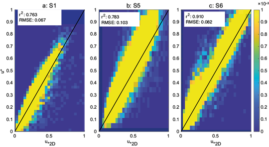
Fig. 4 PDF of actual (3D) friction velocity u* vs. estimated friction velocity u*2D, obtained from 2D velocity components with single rotation, for the sites (a) S1, (b) S5 and (c) S6. Goodness of fit statistics are shown inside the white labels (the thick black line is the 1:1 relationship).
Finally, note that for heterogeneous surfaces and contrasting orography, the planar fit method (Wilczak et al., 2001) is recommended. None of the experimental sites present orography (coastal sites) and only S5 presents a relatively tall canopy (~20 m, see Table I), so a double rotation would be sufficient for calculating fluxes.
7. Conclusions
A simple power law was proposed to estimate the dimensionless friction velocity u * U -1 using only 2D data (horizontal velocity components) from wind measurements at high acquisition rates (of 10 Hz, in this case). This method of estimation was put to test using experimental data coming from six independent experiments carried out in coastal zones of both northern and southern hemispheres (see Table I). Note that at least three of the sites (S1, S3 and S4) show two wind regimes due to sea breeze influence, making the estimation a challenging task.
The results show a very good agreement between the 2D estimate of the friction velocity u *2D and u * (from the 3D EC methodology). The goodness of fit, with r2 > 0.77 in all cases, proves that the methodology can be used at least in flat terrain (homogeneous or complex canopy) like that of coastal zones far from the influence of significant orographic features.
Given the affordability and wide use of 2D anemometers in modern meteorological stations, this study suggests that more estimations of u * could be carried out by research groups and specialists of different disciplines, particularly in developing countries where 3D anemometry is precluded by the high cost of 3D sonic instruments. Moreover, some sites are located only meters from the shoreline, so the method may also be valid to estimate u * above the sea surface (or other bodies of water). More research should be carried out in different experimental conditions. In particular, it would be interesting to test (and adapt) the method in complex orography, urban zones and tall and heterogeneous canopies.

