


 nova página do texto(beta)
 Inglês (pdf)
 Artigo em XML
 Referências do artigo
 Enviar este artigo por email
 Citado por SciELO
  Similares em
SciELO
Similares em
SciELO 
 Permalink
1. Introduction
Droughts were defined in the United Nations Convention to Combat Desertification (UNCCD, 1994) as a phenomenon that is produced naturally when rainfall is considerably lower than the normal recorded levels and, because of its extraordinary characteristic, has considerable impact at the ecological, economic and social levels. Climate change is producing higher temperatures, lower precipitation, and more droughts with higher intensity and duration (Castillo-Castillo et al., 2017)
Wilhite and Glantz (1985) established four types of droughts: meteorological, agricultural, hydrological and socioeconomic. The first three measure drought as a physical phenomenon, while the fourth sees it as a balance of supply and demand. These operational definitions that attempt to give objective criteria of specific applicability (Zargar et al., 2011) were favorably received by the World Meteorological Organization (Ponvert-Delisles and Dámaso, 2016) as well as by Esquivel-Arriaga et al. (2019), Khatiwada and Pandey (2019), Paredes et al.(2015) and Spinoni et al. (2019). Burton et al. (1993) defined seven parameters to characterize droughts: one independent (intensity), four referring to the temporal component (duration, frequency, rate of implantation and temporal spacing), and two referring to the spatial component (extension and dispersion). These parameters can be analyzed using indices to express impact numerically (Valiente, 2001; Zarch et al., 2011). The World Meteorological Organization (OMM and Asociación Mundial para el Agua, 2016) in their manual of drought indicators and indices, describes the 50 most-used indices worldwide and point out that none can be attributed or applied to all types of drought, climate regimes or affected sectors. For this reason, to analyze droughts, it is convenient to consider more than one index with the goal of examining the sensitivity and precision of each one (Ortiz-Gómez et al., 2018).
Numerous indices have been developed in recent years to identify characteristic of meteorological droughts. The most used is SPI (Standardized Precipitation Index) proposed by McKee et al. (1993). To calculate this index, monthly historical registers of precipitation are used to establish a probability of occurrence with positive and negative values that correlate directly with episodes of humidity and drought. Only precipitation data are considered and not temperature, which is important for the water balance when processes of atmospheric warming are included and offers a panorama of evaporative demand. For this reason, Vicente-Serrano et al. (2010) proposed SPEI (Standardized Precipitation Evapotranspiration Index), which includes in its calculation a monthly climate water balance using the difference between precipitation and evapotranspiration as entry data. Both indices enable identification of conditions of deficit and excess humidity at different temporal scales. The corresponding values at a period of three month or less can be useful for basic drought monitoring, values for a period of 6 months or less to monitor effects on agriculture and values for a period of 12 months or more for hydrological effects (SMN, 2019).
Mishra and Singh (2010) mention that in recent years droughts have had higher peaks and severity levels superior to those registered in the past century, as well as shorter intervals of occurrence, signaling climate change. Droughts are insidious natural hazards that pose serious challenges, and their study, identification, and monitoring of their main characteristics have become integral parts of planning, preparation and mitigation at local, regional and even national scales (Lobato-Sánchez, 2016). CONAGUA (2013) identified a long hydrological drought in the Sonora Basin, from 1996 to 2009. Navarro and Moreno (2016) mentioned that the reservoirs “Abelardo Rodriguez” and “El Molinito” have been below the operational level between 1998 and 2014, levels that are not enough to supply water for the City of Hermosillo, Sonora.
Thus, the objective of this study was to analyze meteorological drought temporally and spatially in middle and upper regions of the Sonora River Basin, Mexico, for the period 1974 to 2013 using SPI and SPEI indices at scales of 3, 6, 12 and 24 months. The importance of this study resides in the detailed analysis of the drought described by CONAGUA (2013), highlighting the dramatic situation in northern of Mexico over several years. The study responds to the recommendation of the Drought Monitor with SPI to develop a more detailed study by economic regions. The Sonora basin has experienced an increase in population in recent years and, thus, in water demand by the population and agriculture.
2. Materials and methods
2.1 Description of the study area
The Sonora River basin is located in the northeast-central part of the state of Sonora, bounded by the geographic coordinates 28º5’19.23” and 30º59’18.56” N and 109º52’8.92” and 111º37’52.81” W, and covering an area of 26,827 km2. The current study includes only middle and upper regions of the basin, 21,220 km2 (Fig. 1).
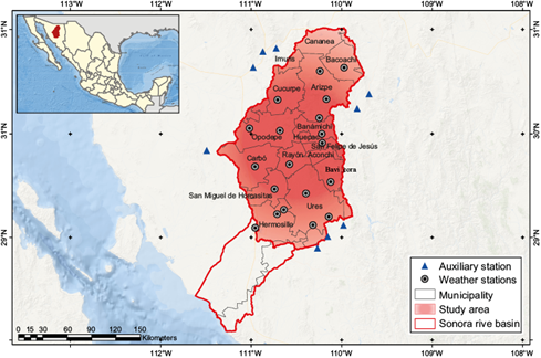
Mean annual precipitation varies from 300 to 600 mm; the highest values occur toward the northwestern part of the study area and to the south in areas of the Sierra Madre Occidental. Most of the rain falls in summer, associated with the North American Monsoon. However, there are also significant rainfall events in winter, resulting from the impact of extratropical cyclones. Mean annual temperatures range between 12 and 24 ºC (CONABIO, 2020); the lowest values occur in the highest mountainous areas of Cananea, Los Ajos and Aconchi mountain ranges. The municipalities included totally or partially in the study area are Aconchi, Arizpe, Bacoachi, Banámichi, Baviácora, Cananea, Carbó, Cucurpe, Hermosillo, Huépac, Imuris, Opodepe, Rayón, San Felipe de Jesús, San Miguel de Horcasitas and Ures, with a total population estimated at 973,800 by the inter-census survey (INEGI, 2015).
2.2 Climatic information used
The series of monthly data on precipitation and maximum and minimum temperatures from a total of 29 stations were obtained from the network of weather stations of the Servicio Meteorológico Nacional (SMN, 2019) for the period 1974 to 2013, that is, 40 years of information. Of these stations, 19 are within the study area and 10 are nearby (Fig. 2).

2.3 Estimation of missing data
The series of data with climate information (precipitation and maximum and minimum temperatures) were not complete during the study period, and it was necessary to estimate the missing data. The method of Inverse Distance Weighting (IDW), or the US National Weather Service method, suggested by the World Meteorological Organization (OMM, 2011), was applied. According to Campos-Aranda (1998), the missing data of a station can be estimated based on observed data of the four (preferably), three or two closest stations. Equations 1 and 2 present the formulas that are applicable for this method.
where Wi is equal to the reciprocal of the square of the distance (d) given in km between each neighboring station with the known data (Di) and the station missing the data (Dx).
2.4 Regionalization of the study area
For the spatial analysis of droughts, first, the climatological data were subjected to meticulous quality control in terms of their continuity, variability and magnitude. When the missing data were estimated with the IDW method to complete the series, the continuity criterion was satisfied. Variability and magnitude of the data were estimated using three standard deviations above or below the mean value of the variable to enable identification of suspicious data, which were analyzed and compared with records of neighboring stations and their validity determined or corrected, as suggested by Cuadrat et al. (2013) and Ravelo et al. (2014).
Homogeneous precipitation regions were determined by grouping meteorological stations so that they would share similar patterns in annual precipitation, using two complementary methodologies. First, mean annual isohyets were plotted manually on the digital elevation model, following the graphic method described by Gómez et al. (2008) where mean annual precipitation, orographic characteristics and wind systems that impact the study area are contemplated. And second, Principal Components Analysis (PCA) was performed using the statistical software RStudio (2018) with the aim of representing the 19 stations by a smaller number (Mallants and Feyen, 1990). Using linear combinations of the original data, the variables, factors, or principal components (PC) that explained successively most of the total variance were calculated (Urrutia and Lemus, 2010). Therefore, a matrix of 19 x 40 was generated, corresponding to the 19 weather stations and the 40 mean annual precipitation records. Finally, with PC1 and PC2, a cluster analysis was performed with Euclidean distance as the method for generating the similarity matrix required for grouping the stations by Partitioning Around Medoids (PAM), also known simply as k-medoids. The advantages of the method are discussed by Estarelles et al. (1992) and Reynolds et al. (2006).
2.5 Analysis of meteorological droughts
There is a wide variety of indices and equations to quantify a drought and characterize it by intensity, duration and frequency. In our study, SPI (Standardized Precipitation Index) and SPEI (Standardized Precipitation Evapotranspiration Index) were calculated at temporal scales of 3, 6, 12 and 24 months for the time series spanning from January 1974 to December 2013.
SPI was calculated following the methodology developed by McKee et al. (1993), using monthly historical records of precipitation (P) to establish a probability of occurrence by fitting them to a gamma distribution. The fitted values are transformed to a normal distribution.
Calculation of SPEI followed the methodology of Vicente-Serrano et al. (2010) where the temperature component is included to enable estimation of evapotranspiration (ETP). ETP is subtracted from precipitation, generating a climatic water balance (P-ETP); this water balance is fit to a log logistic distribution, to later transform it to a normal standard distribution.
Evapotranspiration was calculated by the Hargreaves method modified by Droogers and Allen (2002), which contemplates average monthly temperature (T avg ), computed as the difference between maximum and minimum temperatures, both in degrees Celsius , precipitation in mm (P), difference between maximum and minimum temperature (TD), and radiation in MJm -2 d -1 (RA). Expression (3) represents this reference evapotranspiration (ET o ).
Radiation, RA, resulted from the equation proposed by the United Nations Food and Agriculture Organization (Allen et al., 2006).
The temporal scale used indicated the accumulated period of the input variable (P for SPI and P-ETP for SPEI) to calculate each index. Thus, for the scale of three months, the cumulative input variable of the month of interest and the two previous months is considered. For the scale of six months, the cumulative would be the month of interest plus the five previous months, and so forth.
The SPI and SPEI values, being standardized, can correlate with episodes of humidity and drought. The results are interpreted based on the categories used by the Drought Monitor of Mexico (DMM), whose principal objective is to describe drought evolution in terms of magnitude and spatial extension (Lobato-Sánchez, 2016) and is part of the North American Drought Monitor (NADM) (Table I).
Table I Categories of drought intensity of the North American Drought Monitor.
| Range | Code | Category |
| SI ≥ 2.0 | W4 | Exceptionally humid |
| 1.6 ≤ SI < 2.0 | W3 | Extremely humid |
| 1.3 ≤ SI < 1.6 | W2 | Severely humid |
| 0.8 ≤ SI < 1.3 | W1 | Moderately humid |
| 0.5 ≤ SI < 0.8 | W0 | Abnormally humid |
| -0.5 < SI < 0.5 | N | Normal conditions |
| -0.8 < SI ≤ -0.5 | D0 | Abnormally dry |
| -1.3 < SI ≤ -0.8 | D1 | Moderately dry |
| -1.6 < SI ≤ -1.3 | D2 | Severely dry |
| -2.0 < SI ≤ -1.6 | D3 | Extremely dry |
| SI ≤ -2.0 | D4 | Exceptionally dry |
SI = Standardized index of drought (SPI, SPEI)
SPI and SPEI were calculated with the software SPEI.R for the RStudio program (2018) developed by Begueria and Vicente-Serrano (2017).
Once time series of SPI and SPEI for each of the 19 weather stations were calculated and categorized, the results were aggregated by homogeneous precipitation regions (isohyets). Droughts were identified from the series of aggregated values at different temporal scales, as well as their intensity, duration, frequency, and trend. Intensity was determined based on the categories in Table I. Duration was estimated based on initial and final dates of those indices. Frequency was determined with the number of times that category occurred (Fig. 9). Trend was estimated by linear regression of SPI and SPEI and was plotted as the average slope of both tendencies (Fig. 5, 6, 7 and, 8).
3. Results and discussion
3.1 Regionalization of the study area
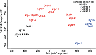
Weather stations were grouped according to mean annual precipitation into: group 1 (300 to 400 mm), group 2 (400 to 500 mm) and group 3 (500 to 600 mm). A correlation matrix between stations was constructed, with values ranging between 0.30 and 0.84, with a mean of 0.62, and a determinant of 2.22 10-11. According to Urrutia and Lemus (2010), if a low determinant value different from zero is obtained, it indicates high intercorrelations between variables (stations), which is our case, and gives rise to factorial analysis of the principal components (PC). Figure 2 shows that the first two PC are the most important, explaining 35.28 % and 14.80 % of the total variability between stations, with respect to mean annual precipitation. This previous conclusion is based on Vicario et al. (2015), who conducted a study with series of monthly precipitation data from 15 stations in the provinces of Córdoba, Santa Fe and Entre Ríos, Argentina for a period of 30 years. Their results revealed that PC1 and PC2 explained 75.1 % of the observed variability between the stations and annual mean precipitation. Urrutia and Lemus (2010) found that the first two components explained 74 % of the variance when they determined homogeneous patterns of temperature in six stations of the Department of Chocó, Colombia.
Figure 3 shows the dispersion diagram from the cluster analysis of the stations obtained from PC1 and PC2 grouped according to the behavior patterns of average annual precipitation. The isohyets generated ahead of grouping the 19 stations into k=3 groups were taken as reference. Vicario et al. (2015) analyzed physical and pluviometric characteristics of 15 weather stations and also generated three groups with similar behavior; their study differed in that they used the average chain-linking method.
Contrasting results of the methodologies used for regionalization revealed a discrepancy in station 26271-Sinoquipe. With a record of average annual precipitation of 504.5 mm, it was placed in the polygon of isohyets of 500-600 mm (group 3). However, the PCA placed it in group 2, where we finally left it after analyzing its geographic location and the pluviometric characteristic of the series, redefining the corresponding isohyet.
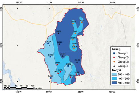
Groups 1 and 3 consist of four stations each, and group 2 contained eleven. This last group was divided into two subgroups (2a and 2b), according to the physiography of the site. Stations in groups 1 and 2a are found within the physiographic province of the Sonora plains, while group 2b and 3 are in the physiographic region of the Sierra Madre Occidental, with the particularity that group 2b is in the intermountain valleys that form the Aconchi, Cananea and Los Ajos mountain ranges. The list of weather stations analyzed and the groups to which they belong are presented in Table II and Figure 4 locates them spatially within the generated isohyets.
Table II Selected weather stations in the study area.
| Station | Altitude | Latitude (N) | Longitude (W) | P (mm) | Tmax (ºC) | Tmin (ºC) | Est. Dat. ( %) | Group | Isohyet (mm) | |
| 26139 | Hermosillo II | 221 | 29º05’56’’ | 110º57’14’’ | 363.5 | 32.2 | 17.7 | 0.3 | 1 | 300 - 400 |
| 26121 | Ures | 385 | 29º25’37’’ | 110º23’31’’ | 375.6 | 31.8 | 9.1 | 12.1 | ||
| 26016 | Carbo | 464 | 29º41’03’’ | 110º57’18’’ | 374.6 | 31.2 | 13.0 | 4.9 | ||
| 26074 | Querobabi | 661 | 30º03’02’’ | 111º01’17’’ | 394.0 | 31.2 | 11.3 | 12.1 | ||
| 26032 | El Orégano | 279 | 29º13’48’’ | 110º42’21’’ | 410.6 | 33.8 | 14.1 | 6.9 | 2a | 400 - 500 |
| 26274 | Topahue | 300 | 29º16’15’’ | 110º38’09’’ | 418.6 | 33.1 | 12.9 | 22.4 | ||
| 26180 | El Cajón | 390 | 29º28’19’’ | 110º44’09’’ | 414.2 | 32.1 | 11.7 | 2.3 | ||
| 26244 | Rancho Viejo | 450 | 29º07’37’’ | 110º18’54’’ | 458.6 | 31.1 | 12.4 | 28.1 | ||
| 26199 | Pueblo de Álamos | 589 | 29º12’15’’ | 110º08’25’’ | 498.8 | 30.8 | 11.7 | 15.8 | ||
| 26214 | Huepac | 644 | 29º54’46’’ | 110º12’47’’ | 496.5 | 30.1 | 9.7 | 19.7 | 2b | |
| 26008 | Banamichi | 675 | 30º00’12’’ | 110º12’54’’ | 459.7 | 30.7 | 13.3 | 1.7 | ||
| 26271 | Sinoquipe | 740 | 30º09’20’’ | 110º14’42’’ | 504.5 | 30.5 | 11.6 | 39.8 | ||
| 26005 | Arizpe | 836 | 30º20’08’’ | 110º10’03’’ | 474.5 | 29.4 | 10.0 | 31.9 | ||
| 26007 | Bacanuchi | 1049 | 30º35’56’’ | 110º14’18’’ | 489.1 | 28.0 | 7.4 | 6.2 | ||
| 26145 | Bacoachi | 1049 | 30º37’54’’ | 109º58’12’’ | 465.5 | 28.0 | 8.2 | 35.3 | ||
| 26198 | Mazocahui | 449 | 29º32’26’’ | 110º07’09’’ | 517.6 | 31.4 | 11.2 | 22.1 | 3 | 500 - 600 |
| 26181 | Rayón | 560 | 29º42’38’’ | 110º34’14’’ | 500.5 | 30.6 | 11.8 | 7.7 | ||
| 26241 | Meresichic | 712 | 30º01’50’’ | 110º40’30’’ | 521.8 | 28.5 | 11.0 | 38.9 | ||
| 26025 | Cucurpe | 853 | 30º19’50’’ | 110º42’21’’ | 524.7 | 29.6 | 10.3 | 10.4 | ||
P= Average annual precipitation, Tmax= Average maximum temperature, Tmin= Average minimum temperature, Est. Dat. = Estimated data.
3.2 Analysis of meteorological droughts
The results of the analysis of meteorological droughts are presented by groups of stations (homogeneous precipitation regions) for which the SPI and SPEI historical series of the weather stations were averaged, and series of mean values for the different temporal scales used were obtained.
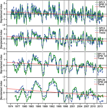
Figure 5 shows the series of average SPI and SPEI values for the stations of group 1 (Hermosillo, Ures, Carbo and Querobabi) where in 1982, 1997, 1999, 2010, 2011 and 2013 at all temporal scales reported droughts of some degree of intensity. Extreme events occurred from August to December 1982 and January 2011 to July 2012, with intervals of exceptional drought in July 1982, March to May and September to October 2011, and in January to June 2012. CONAGUA (2013) reported periods of exceptional drought from 1999 to 2001 and severe drought events in 2004 to 2006 for the Carbo station.
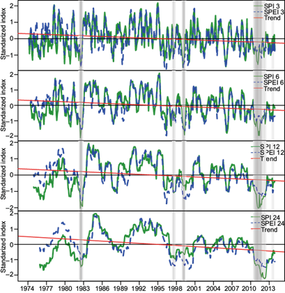
In general, there are great similarities among the behavior of time series of drought indices; that is, drought occurrence is similar when they belong to the same group of weather stations. However, with SPI, on average, 28 % of all the registers were identified with some degree of drought, while with SPEI, it was 30 %. The slope obtained from the time series fit to a linear regression model provided an estimate of the trend; in general, the trend is negative for all temporal scales.
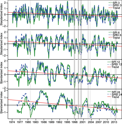
The series of average SPI and SPEI values for group 2a, comprising El Orégano, Topahue, El Cajón, Rancho Viejo and Pueblo de Álamos, are presented in Figure 6. Exceptional drought events were identified in May 1999, March 2006 and June 2011, and droughts of less intensity in 1980, 1987, 1997-2000, 2006, and 2011 at all temporal scales. The longest drought, according to SPI and SPEI at the temporal scale of 24 months, occurred from September 1987 to June 1989 with moderate intensity. CONAGUA (2013) reported that, as of 1996, the hydrometric stations El Cajón and El Orégano registered a decrease in runoff, and the negative trend has continued in recent years.
The time behavior is similar for both indices; on average, 30 % and 32 % of all records indicate some degree of drought for SPI and SPEI, respectively. The latter index evaluates drought periods more rigorously at the end of the series, and the trend estimated by linear regressions was negative for all time series.
Figure 7 presents the temporal series of mean values for the SPI and SPEI indices obtained from averaging values at stations in group 2b (Huepac, Banamichi, Sinoquipe, Arizpe, Bacanuchi and Bacoachi). All time scales indicate simultaneous drought events in 1980, 1997, 1999-2003 and 2011-2013, although of shorter duration than for groups 1 and 2a. In contrast, the longest events detected by both indices at a scale of 24 months occurred from July 1998 to October 2000 and from August 2010 to December 2013, with abnormal to severe intensities in both cases. Within the drought period October 2002 to January 2005, there was an extreme event from July 2003 to February 2004. However, CONAGUA (2013) in reports of the Alto Noroeste Basin Council, indicates that the northwestern part presents extreme drought from March to November 2011, affecting the municipalities of Naco, Santa Cruz, Cananea, Bacoachi, Arizpe, Banámichi, Huépac, Aconchi, Baviacora, Ures, west Altar, Trincheras, Carbó and east Hermosillo. For this group, on average, a moisture deficit of 29 % was registered by SPI and 32 % by SPEI. The trend represented by the slope of the linear regression fit of the data is negative for all cases.
For group 3 (Mazocahui, Rayón, Meresichic and Cucurpe), Figure 8 shows the average SPI and SPEI time series. Note that in 1975, 1976, 1997, 2000 and 2011-2013 there are drought events that synchronize in all time scales. Of the longest events in this group, those that occurred from December 1974 to February 1978 detected in the SPI 12-month series is outstanding. Another outstanding event detected in the SPI 24-month series lasted from August 2010 to December 2013. Both cases had moderate intensity and the 24-month SPEI categorized the event that occurred from July 1976 to June 1977 as extreme. Likewise, in December 2012, CONAGUA (2013) declared 11 municipalities of Sonora a disaster zone because of severe drought, among which was Cucurpe. On average, of the different scales used, SPI detected 142 cases of drought, while SPEI found 138. The trend of the time series is negative, with a less steep slope as compared with the group of stations analyzed previously.
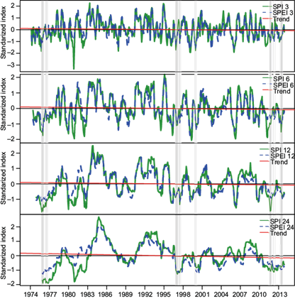
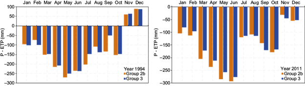
Figure 10 shows how precipitation and evapotranspiration behave in a wet year and in a dry year. Notice how in all months of the dry year (2011) there is a negative water balance (P-ETP). But also notice that even in a wet year (1994), a negative balance is observed. For this reason, we strongly recommend the use of the SPEI index to characterize drought in the Sonora basin.
Table III presents the descriptive statistics by groups of stations of the series of mean SPI and SPEI values at the different scales. The mean is near zero and the standard deviation near one (parameters of a normal standard distribution).
Table III Descriptive statistics of the average time series of SPI and SPEI at different temporal scales by group of stations.
| SPI | Group | SPEI | Group | ||||||||
| 1 | 2a | 2b | 3 | 1 | 2a | 2b | 3 | ||||
| 3 | Drought ( %) | 27.20 | 26.99 | 28.03 | 29.08 | 3 | Drough ( %) | 29.50 | 30.13 | 30.75 | 29.29 |
| Min. | -1.78 | -2.04 | -2.41 | -3.34 | Min. | -1.96 | -1.93 | -2.01 | -1.68 | ||
| Mean | 0.04 | 0.03 | 0.02 | 0.02 | Mean | 0.01 | 0.01 | 0.01 | 0.01 | ||
| S.D. | 0.80 | 0.84 | 0.88 | 0.85 | S.D. | 0.82 | 0.88 | 0.88 | 0.79 | ||
| 6 | Drought ( %) | 29.26 | 27.79 | 28.42 | 28.42 | 6 | Drought ( %) | 29.47 | 31.37 | 33.26 | 27.16 |
| Min. | -2.13 | -2.40 | -2.46 | -2.06 | Min. | -1.97 | -1.75 | -1.89 | -1.75 | ||
| Mean. | 0.01 | 0.00 | 0.00 | 0.00 | Mean | 0.01 | 0.00 | 0.00 | 0.01 | ||
| S.D. | 0.83 | 0.88 | 0.88 | 0.87 | S.d. | 0.82 | 0.88 | 0.88 | 0.79 | ||
| 12 | Drought ( %) | 27.93 | 29.64 | 32.41 | 33.90 | 12 | Drought ( %) | 31.34 | 32.20 | 32.62 | 32.84 |
| Min. | -2.04 | -1.99 | -1.97 | -1.81 | Min. | -1.75 | -1.76 | -1.66 | -1.39 | ||
| Mean. | 0.00 | 0.00 | 0.00 | 0.01 | Mean. | 0.00 | 0.00 | 0.00 | 0.00 | ||
| S.D | 0.84 | 0.85 | 0.84 | 0.87 | S.D. | 0.83 | 0.87 | 0.87 | 0.76 | ||
| 24 | Drought ( %) | 29.32 | 34.14 | 29.10 | 29.54 | 24 | Drought ( %) | 28.88 | 33.92 | 31.51 | 28.45 |
| Min. | -2.23 | -1.52 | -1.72 | -1.89 | Min. | -1.62 | -1.60 | -1.78 | -1.25 | ||
| Mean. | 0.00 | 0.00 | 0.00 | 0.00 | Mean. | 0.00 | 0.01 | 0.00 | 0.00 | ||
| S.D. | 0.87 | 0.85 | 0.83 | 0.90 | S.D. | 0.85 | 0.86 | 0.87 | 0.71 | ||
Drought ( %)= Drought in %, Min.= Minimum, S.D.= Standard deviation.
Table IV lists drought events according to the intensity detected by SPI and SPEI for each group of stations at 3, 6, 12 or 24 months, while in Figure 9 they are expressed in percentage in a frequency graph. In general, moderate droughts dominate in groups 1, 2a and 2b, while group 3 mostly presents abnormally dry conditions.
Table IV Frequency of occurrence of drought events.
| Drought | Group | SPI 3 | SPEI 3 | SPI 6 | SPEI 6 | SPI 12 | SPEI 12 | SPI 24 | SPEI 24 |
| Exceptional | 1 | 0 | 0 | 1 | 0 | 4 | 0 | 8 | 0 |
| 2a | 2 | 0 | 5 | 0 | 0 | 0 | 0 | 0 | |
| 2b | 5 | 1 | 9 | 0 | 0 | 0 | 0 | 0 | |
| 3 | 1 | 0 | 1 | 0 | 0 | 0 | 0 | 0 | |
| Extreme | 1 | 5 | 10 | 10 | 7 | 10 | 2 | 7 | 1 |
| 2a | 9 | 11 | 16 | 9 | 10 | 4 | 0 | 0 | |
| 2b | 12 | 8 | 9 | 9 | 7 | 1 | 2 | 8 | |
| 3 | 9 | 3 | 16 | 1 | 5 | 0 | 17 | 0 | |
| Severe | 1 | 16 | 13 | 15 | 13 | 12 | 14 | 23 | 23 |
| 2a | 23 | 22 | 14 | 28 | 21 | 20 | 10 | 24 | |
| 2b | 16 | 20 | 16 | 22 | 18 | 24 | 15 | 16 | |
| 3 | 18 | 15 | 16 | 12 | 23 | 3 | 10 | 0 | |
| Moderate | 1 | 48 | 52 | 53 | 62 | 61 | 76 | 46 | 63 |
| 2a | 42 | 64 | 55 | 61 | 55 | 77 | 59 | 64 | |
| 2b | 53 | 65 | 60 | 70 | 60 | 79 | 63 | 61 | |
| 3 | 54 | 48 | 43 | 54 | 60 | 68 | 54 | 56 | |
| Abnormal | 1 | 61 | 66 | 60 | 58 | 44 | 55 | 50 | 45 |
| 2a | 53 | 47 | 42 | 51 | 53 | 50 | 87 | 67 | |
| 2b | 48 | 53 | 41 | 57 | 67 | 49 | 53 | 59 | |
| 3 | 57 | 74 | 59 | 62 | 71 | 83 | 54 | 74 |

It should be mentioned that, on average, SPEI detected a higher number of drought events at the different scales, as well as a trend with a pronounced negative slope, which means an increase in intensity and demonstrates the relevance of including variables such as evapotranspiration to study droughts. However, SPI more often characterized exceptional droughts. This behavior was also reported by Serrano-Barrios et al. (2016) when they analyzed droughts in the north Pacific basin between 1961 and 2010. In a similar way, Campos-Aranda (2018), Castillo-Castillo et al. (2017) and Vicente-Serrano et al. (2012) concluded that temperature should be included when studying droughts.
In general, droughts were detected in 1997 and 2011. In 1999 and 2000 important events occurred in most of the study area, with the exception of groups 3 and 1 in the respective years. These results agree with those reported by Sthale et al. (2009), who stated that from 1994 to the early 21st century droughts have been more severe and sustained throughout Mexico. Similarly, Castillo-Castillo et al. (2017) found two periods of extreme drought from 1999 to 2004 and from 2011 to 2012 in the Fuerte River basin located in northwestern Mexico. CONAGUA (2013) reported droughts from 1999 to 2007, analyzing SPI, SPEI and the Palmer index. CONAGUA analyses detected the May-November 2011 droughts, occurring with some degree of intensity in practically 50 % of the country’s territory, affecting agriculture and livestock in the north of Mexico. It is worth mentioning that Eakin et al.(2007) described serious problems of lack of available water in the state of Sonora in the 1990s caused by a decrease in precipitation, and a severe drought was declared. Also, the reports of CONAGUA (2010) and Navarro and Moreno (2016) agree with results presented here.
Finally, it is important to mention that the official Mexican agency responsible for following up the evolution of this phenomenon is the Servicio Meteorológico Nacional (SMN) supported by the Drought Monitor of Mexico (DMM), which is part of the North American Drought Monitor (NADM). DMM methodology is based on estimating and interpreting several indices, including SPI, one of the most frequently used in North America (Velasco et al., 2004). However, our study showed that SPEI was useful and has potential for detection of droughts. While the SMN drought monitor gives a general view of the country, it is better to monitor drought specifically and in detail at basin level to enable better planning when dealing with droughts.
4. Conclusions
The values of SPI and SPEI at different temporal scales in the study area showed drought occurrence in several periods in 1997 and 2011 for all groups of stations in meddle and upper regions of the Sonora River basin. Droughts were identified in 1999 and 2000 in groups 2a and, 2b, while groups 1, 2b and 3 presented some moisture deficit in 2012 and 2013.
The linear fit estimated by regression of the temporal series showed a negative trend throughout the study period, indicating a clear increase in the intensity and frequency of drought events in the study area. The negative trend occurred between 1997 and 2013, coinciding with results reported by different authors and institutions.
The frequency of drought in group 3 was lower, attributed to higher precipitation in these areas associated with the interaction of the mountain systems that force air ascent from the Gulf of California, leading to increased condensation and precipitation development. In contrast, in group 2, located in the intermountain valleys where winds descend and inhibit cloud formation, precipitation decreases and there is greater occurrence of exceptional droughts.
Calculation and interpretation of SPI and SPEI at different temporal scales enables convincing detection of the most important drought events of some intensity. However, because it uses a climate balance (P-ETP), SPEI includes water demand by the atmosphere and reveals a more realistic panorama of water availability in the study zone than SPI, which is based solely on precipitation data. We recommend the use of the SPEI over the SPI, because it explicitly considers temperature and evapotranspiration.
The results obtained in this work are relevant and helpful in future water planning and management for all uses. Future research in this topic and in this area should be directed towards seasonal forecast of droughts to enable advance preparation to reduce and mitigate their effects.

