


 nueva página del texto (beta)
 Inglés (pdf)
 Artículo en XML
 Referencias del artículo
 Enviar artículo por email
 Citado por SciELO
  Similares en
SciELO
Similares en
SciELO 
 Permalink
1. Introduction
Energy production depends on different local factors, such as climate and terrain (Tan and Zhi, 2016). The large availability of water resources in Brazil is used for human consumption, industry, agriculture, and energy production. According to the Energy Research Company (EPE, 2019), renewable resources in Brazil generated 495.290 GWh of electricity in 2018, and almost 80% by hydropower plants.
Adami et al. (2017) estimated the wind energy generated worldwide from 2006 to 2016, indicating an average growth of 23%, and currently representing 3% of the total energy generated worldwide. This growth can be associated with public policies which encourage wind power generation (Adami et al., 2017; Raimundo et al., 2018; Rego and Ribeiro, 2018). Brazil created, through Law Nº 10.438 of April 26 of 2002, the Alternative Energy Sources Incentive Program (PROINFRA) to increase the use of alternative renewable resources to produce energy, especially encouraging wind farms, small hydroelectric power plants, and biomass sources in order to reach 10% of country’s annual electricity consumption by 2022 (Brasil, 2002). In 2018, wind and solar power plants were responsible for, respectively, 9.78% and 0.70% of the total energy production (EPE, 2019).
Minas Gerais (MG) located in southeastern Brazil is the fourth largest state in territorial extension, with an area of ~ 587000 km², a population of ~21 million people and a Human Development Index (HDI) of 0.731. Its main economic activities are: agriculture, livestock, industry, services, power generation, and mining (IBGE, 2018). MG is the fourth state in terms of power generation in Brazil. However, due to the high demand, the production is still insufficient, and for example in 2017, the state generated only 54.3% of its energy demand. A decrease in production in 2014 and 2015 due to an intense drought period (Coelho et al., 2016) contributed an increase on external energy dependence (3.4% per year). Energy production in MG corresponds to 7.35% of the total national production from basically three sources: hydro (79.0%), thermal (19.2%), and solar (1.8%). No energy is produced by wind sources in MG, despite the existence of a wind power plant in the city of Gouveia (Jequitinhonha Valley), but not in operation due to financial reasons (CEMIG, 2019; EPE, 2019). The large seasonal and interannual variability in rainfall rates hinders energy production and, according to the AR5 Synthesis Report from Intergovernmental Panel on Climate Change (IPCC, 2014), climate projections indicate the intensification of weather extremes, placing the hydroelectric system at risk. Due to the severe droughts during 2014 and 2015 in the southeastern region of the country, where 42.13% of the Brazilian population lives (IBGE, 2018), local governments were forced to implement energy rationing and to reduce water distribution for human consumption (Ribeiro, 2017).
Natividade et al. (2017) through the analysis of observations and projections data, identified an increase in the number of dry days in the northern region of MG; meanwhile, Reboita et al. (2018b) revealed an increase of dry consecutive days and a decrease of wet consecutive days in most MG from precipitation projections. Potential Evapotranspiration also shows positive trends directly proportional to temperature trends in MG (Salviano et al. 2016). With higher availability of moisture in the atmosphere, the number of rainfall extreme events can increase. Reboita et al. (2018b) analyzed climate projections for MG and indicated an increase of extreme events mainly in the austral summer. All these climate factors directly affect water level in reservoirs.
Towers for wind energy generation need to be at least 100 m tall, to avoid the drag effect of the wind at the surface. Moreover, wind intensity projections at 100 m using the RegCM4 regional climate model for MG (RCP8.5 scenario) showed only slight diffe- rences between the near future (2020 to 2050) and the present (1979-2005) of ~ 0.5 m s-1 depending on the season and state region. Differences between the present and the far future, however, presented variations of around 1 m s-1 (Reboita et al., 2018a). These results may indicate that wind patterns are less vulnerable to climate change when compared with other weather variables and it could be a promising source of electricity production in the state, complementing the hydroelectric source (Reboita et al., 2018a).
The wind resource assessment and characterization of a given region needs to consider information about the availability and variability of local winds. The Wind Power (2019) highlights that minimum extreme intensity values (less than 4 m s-1) may not move the turbines; speeds between 13 and 25 m s-1 do not generate increases in power density; and maximum extremes (higher than 25 m s-1) can cause severe structural damage to the towers. Moreover, small variations in wind intensity generate significant variations in energy production since the power density is proportional to the cube of the wind speed (Emeksiz and Cetin, 2019).
The approval and installation of wind power projects require initial studies with at least five years of data from weather stations at 50, 70, and 100 m which, in general, are scarce in Brazil (Cancino-Solorzano and Xiberta-Bernat, 2009). The Wind Atlas of the MG Energy Company used the Mesomap system, complemented by data from anemometric measurement stations, to assess wind energy potential throughout the state. The Mesomap system is a set of atmospheric simulation models that consists of the Mesoscale Atmospheric Simulation System (MASS) with a horizontal resolution of 3.6 km x 3.6 km (CEMIG, 2010). The results show wind in MG reaches values above 8 m s-1 during the winter and mainly in the northern region. However, in the absence of observations, the use of Numerical Weather Forecast (NWF) models can help in the decision-making process. Its results also can help to identify possible new viable sources of renewable energy and contribute to the diversification of state production. Therefore, this study aims to assess the ability of the Global Forecasting System (GFS) reanalysis product to estimate the potential for wind power generation, using the state of MG - Brazil from 2013 to 2017 as an example. The GFS model results data are available through the National Ocea- nic and Atmospheric Administration (NOAA, 2018) since 1980; therefore, the methodology presented in this study can be applied to other regions where observations are scarce or unavailable.
2. Methodology
2.1 Data
The GFS is a global weather forecasting model (NOAA, 2018), developed and operated by the National Centers for Environmental Prediction (NCEP), which uses the Gridpoint Statistical Interpolation (GSI) as a global analysis scheme (Rajagopal et al., 2007; Prasad et al., 2011). The GSI is included in the Global Data Assimilation and Forecasting (GDAF) system at National Centre for Medium Range Wea- ther Forecasting (NCMRWF) and the assimilation runs are performed using the six-hour intermittent method (the system has access to a database observed four times a day), where three main interactions are carried out (between predictions and observations) and the analyses are used as initial conditions for subsequent predictions (Prasad et al., 2011; 2017). The results of the GFS analyses (meteorological term applied to indicate a model result that is not a forecast) were used with horizontal resolution of 0.5 degrees, 64 vertical levels, and six-hour frequency (0, 6, 12 and 18 UTC). The period considered was from 2013 to 2017 for the entire state of MG. From the zonal (UGRD) and meridional (VGRD) components, the intensities (m s-1) and directions (º) of the wind were obtained every six hours. Daily and monthly averages were also calculated.
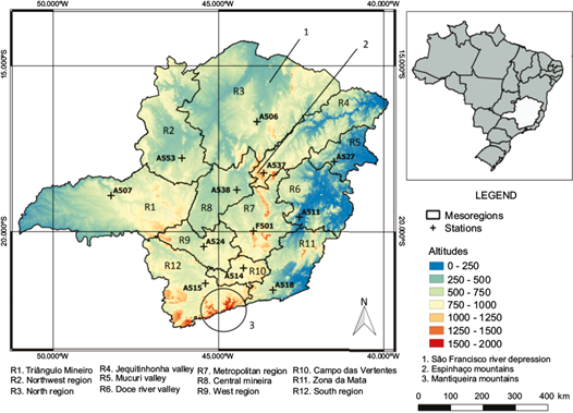
To verify how the GFS analyses represent the weather conditions in the state, observations at 10 m from twelve weather stations between 2013 and 2017 were used (Table I). These weather stations belong to the National Institute of Meteorology (INMET) and were chosen according to the mesoregions of the State of MG. These regions were defined, based on economic and social similarities, by the Brazilian Institute of Geography and Statistics (Brazilian Institute of Geography and Statistics - IBGE, 2018). For comparison, GFS data were extracted from the nearest grid points of the weather stations. Figure 1 shows the location of the stations and terrain elevation through the state. In the south, the altitude is higher, characterized by the Mantiqueira Mountains (Serra da Mantiqueira). In the north the altitude is more heterogeneous, with the Espinhaço Mountains (Serra do Espinhaço) and the São Francisco River Depression, for example (CEMIG, 2010).
Table I List of weather stations.
| Region | Code | Station | Latitude | Longitude |
| Campo das Vertentes | A514 | São João Del Rei | 21.10ºS | 44.25ºW |
| Central Mineira | A538 | Curvelo | 18.74ºS | 44.45ºW |
| West | A524 | Formiga | 20.45ºS | 45.45ºW |
| Northwest | A553 | João Pinheiro | 17.78ºS | 46.11ºW |
| North | A506 | Montes Claros | 16.68ºS | 43.84ºW |
| Metropolitan Region | F501 | Belo Horizonte | 19.98ºS | 43.95ºW |
| South | A515 | Varginha | 21.56ºS | 45.40ºW |
| Triângulo Mineiro | A507 | Uberlândia | 18.91ºS | 48.25ºW |
| Jequitinhonha Valley | A537 | Diamantina | 18.23ºS | 43.64ºW |
| Zona da Mata | A518 | Juiz de Fora | 21.76ºS | 43.36ºW |
| Mucuri Valley | A527 | Teófilo Otoni | 17.89ºS | 41.51ºW |
| Doce River Valley | A511 | Timóteo | 19.56ºS | 42.56ºW |
(the acronym was explained in the text): Source: Adapted from INMET (2018)
2.2 Statistical Analyses
The evaluation of the wind speed and direction from GFS results was made through graphs and wind roses. Data obtained by weather stations were also compared with model results (at 10 m). Seasonal, monthly, and diurnal variability analyses of wind speed data were also performed. The diurnal cycle variability is important, as it allows the identification of the time when the wind reaches its highest intensity in a given location; in general, efficient production of wind energy will occur when the highest wind speed is recorded. The average 6-hour and monthly wind profiles from observational data and GFS results were also compared.
The frequency distribution of wind intensity can be represented by the Weibull distribution. This distribution has been adjusted to the GFS analysis and observational data to identify the constancy of wind intensity around an average value. Note that the Weibull distribution depends only on two parameters: the “k” shape and the “c” scale (Chandel et al., 2014; Wais, 2017). These parameters were obtained through Equations 1 and 2 respectively, where σ is the standard deviation, v̅ is the average velocity and the gamma function (Γ). The parameter “k” is related to the shape of the wind speed distribution (dimensionless), and it is strictly related to the standard deviation of wind speed data while the parameter “c” is directly related to the average wind speed (ms-1) (Wais, 2017; Katinas et al., 2018). The parameters of the Weibull distribution are a simple way to compare different datasets.
2.3 Wind Power Density (WPD)
Kalmikov (2017) indicates that seasonal mean power density (WPD) values are more advantageous than wind speed values, especially when comparing locations with asymmetric frequency characteristics, given the sensitivity of WPD to wind variations. WPD (W m-2) was calculated from the GFS using Equation 3, widely used nowadays. This methodo- logy was also applied by Hennessey Jr. (1977), Patel (2006), Silva et al. (2016), Reboita et al. (2018a), and Emeksiz et al. (2019), and considers the air density (ρ = 1.225 kg m-3) and the wind speed (v):
Calculating WPD per unit area (W m-2) and considering the maximum power coefficient (cp) imposed by the Betz Law. The Betz Limit shows the maximum efficiency can be obtained from a wind turbine is 59.3%, which means the ratio between the input and output of the wind turbine is one third (Manwell et al., 2009; Burton et al., 2011). Thus, cp = 0.593.
Elliotti et al. (1991) previously used WPD = 0.955 ρv 3 to calculate tables of wind power density classification for winds measured at 10 and 50 m. Table II is a modified version of the one presented in Elliotti et al. (1991), comparing original WPD estimates with those calculated from Eqn. 3 and including data at 100 m.
Table II Classification of wind power density, where v is the wind speed (ms-1) and WPD is the wind power density (W.m-2). The WPD 1 correspond to values for 10 and 50 m calculated in the original study based on the Rayleigh distribution (Elliotti et al., 1991). WPD 2 values were calculated using Equation 3.*Values calculated for 100 m, maintaining the calculation standard of the original publication.
| Classes | 10 m | 50 m | 100 m | ||||||
| v | WPD 1 | WPD 2 | v | WPD 1 | WPD 2 | v* | WPD 1* | WPD 2* | |
| 1. Poor | 0-4.4 | 0-100 | 0-52.2 | 0-5.6 | 0-200 | 0-107.6 | 0-6.2 | 0-280.6 | 0-146.9 |
| 2. Marginal | 4.4-5.1 | 100-150 | 52.2-81.3 | 5.6-6.4 | 200-300 | 107.6-160.6 | 6.2-7.2 | 280.6-436.9 | 146.9-228.7 |
| 3. Moderate | 5.1-5.6 | 150-200 | 81.3-107.6 | 6.4-7.0 | 300-400 | 160.6-210.1 | 7.2-7.9 | 436.9-578.4 | 228.7-302.8 |
| 4. Good | 5.6-6.0 | 200-250 | 107.6-132.3 | 7.0-7.5 | 400-500 | 210.1-258.4 | 7.9-8.5 | 578.4-711.4 | 302.8-372.5 |
| 5. Excellent | 6.0-6.4 | 250-300 | 132.3-160.6 | 7.5-8.0 | 500-600 | 258.4-313.6 | 8.5-9.0 | 711.4-863.4 | 372.5-452.0 |
| 6. Excellent | 6.4-7.0 | 300-400 | 160.6-210.1 | 8.0-8.8 | 600-800 | 313.6-417.4 | 8.0-9.9 | 863.4-1129.7 | 452.0-591.5 |
| 7. Excellent | >7.0 | >400 | >210.1 | >8.8 | >800 | >417.4 | >9.9 | >1129.7 | >591.5 |
3. Results and Discussion
3.1 Wind Spatial Distribution
Wind seasonal averages at 10 and 100 m are shown in Figures 2 and 3, respectively. Wind averages vary over the seasons due to intensification or weakening of atmospheric systems, mainly associated with the South Atlantic Subtropical Anticyclone (SASA), South Atlantic Convergence Zone (SACZ), and Frontal Systems (Reboita et al., 2010; Reboita et al., 2015; Reboita et al., 2019).
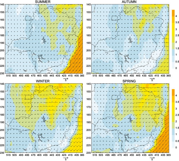
Fig 2 Wind seasonal average at 10 m from 2013 to 2017. Intensity (ms-1) is shaded and vectors indicate wind direction (º).
GFS indicates that, in general, the wind at 10 m (Fig. 2) has low intensity, not exceeding 2 m s-1 in the south and 3.5 m s-1 upstate. However, the wind speed at 100 m (Fig. 3) shows higher values due to surface roughness which tends to decrease with height. The northern portion of the State shows wind speed average at 10 m between 1 and 2.5 m s-1 during austral summer and autumn; at 100 m, average values between 3.5 and 4.5 m s-1 were found, respectively. During winter and spring, wind-speed values increase from 2.5 to 3.5 m s-1 (at 10 m) and from 4 to 6 m s-1 (at 100 m). A similar pattern is seen throughout the state. The wind speed at 100 m is equal to the minimum threshold for energy generation during winter and spring (dry season), which is 4 m s-1 (for small electric wind turbines) and wind turbines on a scale of public utility and 6 m s-1 (wind farms on larger scales), according to Culture Change (2017) and The Wind Power (2019). The North (R3, see map in Fig. 1) and Jequitinhonha Valley (R4) regions have the highest wind intensities, agreeing with CEMIG (2010). Higher wind speed values during winter and spring indicates a possible anti-correlation between wind and precipitation which presents minimum values in these seasons (Silva and Reboita, 2013; Reboita et al., 2015; Reboita et al., 2017; Reis et al. 2018) and reinforces a positive factor for the expansion of wind power in the state energy matrix. Wind farms would have greater production in months with low operation of the hydroelectric power plants and thus, energy production would be complementary between the two sources.

Fig. 3 Wind speed seasonal averages at 100 m (ms-1) from 2013 to 2017. Intensity (ms-1) is shaded and vectors indicate wind direction (º)
In agreement with ERA-Interim reanalysis data and RegCM4 model results by Reboita et al. (2018a), wind density values show significant differences between northern (R3) and southern (R12) regions of MG and higher wind speed values during winter and springtime. However, ERA-Interim data presented a higher contrast between those regions; while the northern region showed wind intensity lower than 6 m s-1, the southern region presented values lower than 3 m s-1, matching those of the GFS analysis.
Another important factor is that the average wind speed is less than the maximum limit, favouring eolic energy generation throughout the day and seasons, minimizing possible structural problems. Results in Figure 4 do not differ significantly from those reported by Paula et al. (2017): wind speeds varying from 0.8 to 5.5 m s-1, more intense in winter and in northern MG. It is worth mentioning that Paula et al. (2017) used only data from meteorological stations, and, in addition, authors performed vertical extrapolation of wind speed data to estimate values at 100m.

Fig. 4 Wind roses determined for the period 2013-2017 in stations: (A) Belo Horizonte, (B) Curvelo and (C) Formiga, representing: (1) observed data, (2) GFS data (10 m) and (3) GFS data (100 m). The legend is in ms-1.
The wind direction pattern at 10 m and 100 m is mainly influenced by SASA, which plays an impor- tant role in the climate of South America. Moreover, as reported by Reboita et al. (2019), the SASA area expands to south and west in climate projections compared to its current climate position. This expansion of SASA may affect weather conditions, modifying the frequency of dry periods, and directly impacting the energy sector in southeastern Brazil. The SASA gains strength in winter and extends to the western Atlantic Ocean, hampering convective movements and cold fronts in southeastern Brazil and, consequently, reducing precipitation rates (Reboita et al., 2015; Reboita et al., 2017). Therefore, there is a possible complementarity between wind and hydroelectric power plants mainly during the winter (dry season) when hydroelectric power plants operate at low capacity.
3.2 Analysis of predominant wind direction
Wind direction from GFS results at 10 m was compared with observed wind direction data at twelve sites. Wind roses are presented for the predominant wind direction from GFS at 100 m. Emeksiz et al. (2019) indicate the wind direction analysis can provide information to support the decision of where to install the wind turbines in order to maximize its efficiency. Table III shows that observational data at 10 m from stations presented variable directions. In contrast, the GFS data at both 10 and 100 m, presented predominant northeast-southeast direction, while showing differences in wind speed, and not satisfactorily simulating the observed direction at 10 m.
Table III Predominant wind direction.
| Station | Observed (10 m) | Simulated (10 m) | Simulated (100 m) |
| Belo Horizonte | NE - SE | NE - SE | NE - SE |
| Curvelo | NE - SE | NE - SE | NE - SE |
| Diamantina | E - S | NE - SE | NE - SE |
| Formiga | NE - SE | NE - SE | NE - SE |
| Juiz de Fora | N - E | NE - SE | NE - SE |
| João Pinheiro | E - S | NE - SE | NE - SE |
| Montes Claros | N - E | NE - SE | NE - SE |
| São João Del Rei | E - S | NE - SE | NE - SE |
| Timóteo | NW - NE | NE - SE | NE - SE |
| Teófilo Otoni | NE - E | NE - SE | NE - SE |
| Uberlândia | N - E | NE - SE | NE - SE |
| Varginha | E - S | NE - SE | NE - SE |
As an example, Figure 4 shows that Belo Horizonte (A), Curvelo (B) and Formiga (C) stations have a similar predominant wind direction at 10 and 100 m. In contrast, wind direction from GFS are more homogenously distributed. In general, the wind turbines would be better positioned in the NE-SE direction, where they would experience the highest frequency of winds.
Moreover, Figure 4 indicates that wind direction patterns from GFS do not show significant differences between 10 and 100 m. This absence of changes in the wind direction with height over cities (most of the stations analyzed are located in or close to urban centers) suggests little or no influence of urbanization. However, it is well known that urbanization increases energy loss at the surface, affecting both the intensity and the prevailing wind direction. Large urban centers, which expand as population grows, undergo processes that involve changes in land use and occupancy which, in turn, modify surface roughness conditions. GFS is unable to represent terrain conditions adequately well in the interpolation process of wind direction in these regions.
3.2 Wind variability patterns
In terms of seasonal variability, wind speed averages in MG are lower during austral summer and fall, coinciding with higher rainfall rates which guarantee that hydroelectric plants can operate at maximum efficiency. Wind speed averages are higher between July and October (austral winter) reinforcing potential complementarity between higher wind and lower precipitation. Thus, during the dry season, stronger winds can help meet the state’s energy demand. At 100 m, cities as Uberlândia, Montes Claros, and Teófilo Otoni (located in the Triângulo Mineiro (R1), North region (R3), and Mucuri Valley (R5), respectively) presented wind speed averages close to 6 m s-1. Observations and results from GFS at 10 m show values between 1.5 and 3 m s-1. The lowest wind speed averages were registered between February and May.
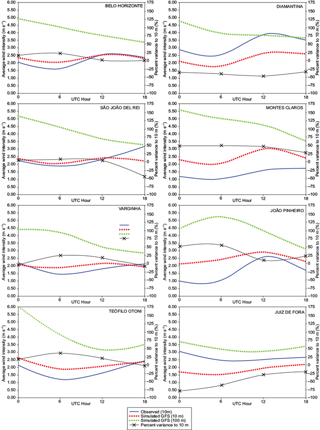
The comparison between observed and GFS profiles showed similar patterns in most sites (Fig. 5). Best results were found for Belo Horizonte, São João del Rei and Varginha (municipalities where the stations are located in areas with few obstacles, in general, with undergrowth or agricultural plantations), while greater differences can be observed in Diamantina, Montes Claros and Juiz de Fora where stations are located in areas with larger obstacles (such as high rocks in the case of Diamantina) or residential areas (in Montes Claros and Juiz de Fora). In general, the GFS model overestimated values at 10 m when compared to the observations, except in Diamantina, Juiz de Fora and São João Del Rei (also shown by the percentage changes).

Fig. 5 Average monthly wind profile (ms-1) observed at 8 selected sites (at 10 m, blue line) compared with derived GFS values at 10 m (red dots) and at 100 m (green dots). The black line corresponds to the variance of the observed wind at 10m.
As for diurnal wind speed variability, at 10 m the highest speed was recorded at 12 h and the lowest between 0 h and 6 h, in agreement with the diurnal cycle of the Earth’s surface temperature. At 100 m, the highest speed occurred between 0 h and 6 h (night and dawn) and decreased throughout the day. Observed and GFS profiles show similar patterns at most sites (Fig. 6). The GFS model also overestimated values at 10 m when compared to the observed values, except in Diamantina and Juiz de Fora.
3.4 Weibull Distribution
Statistics are used in wind studies to represent wind variability and evaluate its evolution, with respect to average values and the probability of occurrence of extreme values, and facilitate the comparison between data sets. When the Weibull shape parameter k presents high values, it indicates little variability of the wind speed around an average value, whereas the parameter c indicates the average value of the data. For observations at 10 m at all sites, k values ranged between 1 and 2.16. The values of c presented greater variability, as can be seen in Table IV. According to Patel (2006), when k is equal or close to 1 the Weibull distribution approaches an exponential distribution, as in the case of Montes Claros (top-right panel in Fig. 8, blue line), and it indicates that most days registered calm or very weak winds. When k values equal to or close to 2 (Rayleigh distribution), such as in Belo Horizonte, Diamantina, Juiz de Fora and Uberlândia, present standard distributions of wind speeds (found in most places), and in these cases most days have speeds below the average speed.
Table IV Parameter values k (distribution format, Eqn. 1) and c (average speed, Eqn. 2).
| Station | Observed (10 m) | Simulated (10 m) | Simulated (100 m) | |||
| k | c (m s-1) | k | c (m s-1) | k | c (m s-1) | |
| Belo Horizonte | 2.05 | 2.42 | 2.86 | 2.57 | 2.59 | 4.62 |
| Curvelo | 1.44 | 2.15 | 2.42 | 2.21 | 2.16 | 3.98 |
| Diamantina | 2.16 | 3.67 | 2.73 | 2.59 | 2.79 | 4.57 |
| Formiga | 1.50 | 2.25 | 2.52 | 2.58 | 2.24 | 4.62 |
| João Pinheiro | 1.53 | 2.87 | 2.67 | 2.78 | 2.34 | 4.86 |
| Juiz de Fora | 2.08 | 3.18 | 2.31 | 2.09 | 2.29 | 3.77 |
| Montes Claros | 1.39 | 1.73 | 2.58 | 2.78 | 2.64 | 5.30 |
| S. João Del Rei | 1.65 | 2.74 | 2.57 | 2.56 | 2.29 | 4.65 |
| Teófilo Otoni | 1.54 | 2.20 | 2.81 | 2.53 | 2.39 | 4.72 |
| Timóteo | 1.70 | 1.37 | 2.50 | 1.94 | 2.31 | 3.54 |
| Uberlândia | 1.90 | 2.24 | 2.22 | 2.78 | 2.27 | 4.97 |
| Varginha | 1.81 | 2.22 | 2.39 | 2.26 | 2.09 | 4.10 |
All observational datasets showed positive asymmetries, where the modal value < median of the values < average speed value (Pishgar-Komleh et al., 2015). Similar calculations with the GFS datasets at 10 m and 100 m, result in values of k between 2 and 3 (Fig. 7 and 8). Also according to Patel (2006), distributions with k = 3 (as in Diamantina and Belo Horizonte) are similar to a normal distribution, where the number of strong winds is equal to the number of light winds (symmetric with respect to the mean). The parameter c, in general, was close to 3 ms-1 (10 m) and 4 ms-1 (100 m). Analyses carried out by Ramos et al. (2018) show distribution patterns as positive examples for eolic energy generation, as they detect only minor problems with the change of the wind (winds with less variability).

Fig. 7 Weibull distributions calculated for observed wind speed at 10 m (blue line) at selected 6 sites for the period (2013 - 2017) and GFS values at 10m (red line) and 100m (green line).

Results from observations and GFS show that the frequency of occurrence of extreme events greater than 8 ms-1 is less than 1%. The analysis show that the winds have acceptable annual values of k but are lower than those found in regions with high wind potential, such as the Brazilian Northeast (with k values equal to or greater than 6) (CRESESB, 2001).
An accurate and reliable assessment of wind resources plays an important role in the effective use of wind energy (Shamshirband et al., 2016). Given the variety of studies carried out that confirm the efficiency of the Weibull distribution (Shoaib et al., 2017; Katinas et al., 2018; Souza et al., 2019) in wind studies, it can be concluded that the results presented show that wind intensity data, provide relevant general information on wind variability.
3.5 Wind Power Density (WPD)
Values of WPD depend on the wind turbine model with different power coefficients (cp), as expressed in Eqn. 3. Figure 9 presents the seasonal average of WPD at 100m, considering the air density equal to 1,225 kg m-3. The left column in Fig. 9 disregards the maximum power conversion estimated by the Betz Law, which shows maximum yield from a wind turbine to be 59.3% (Manwell et al., 2009). WPD results show lowest values during summer and fall, below 70 W m-2 with higher values in the north and lower values in the south of MG. During winter and spring values are higher, reaching 150 Wm-2 in the north region. The right column (Fig. 9) shows WPD seasonal average at 100 m, considering the maximum power conversion estimated by the Betz Law, resulting in an approximate 60% reduction compared to the right column. As cp values depend on the wind turbine chosen, such reduction is variable, and it should be taken into account in the calculations as it influences the relationship between wind speed and generated power density.

Fig. 9 WPD (Wm-2) at 100 m, from 2013 to 2017. Left column: WPD without considering cp. Right column: WPD considering the maximum cp value (59.3%) of the Betz Limit (Manwell et al., 2009).
WPD results have a high sensitivity to wind speed; therefore, its values are higher when wind speed values are higher. Regions with wind speed above 4.5 ms-1 at 100 m have higher wind energy generation potential. However, the values are low when compared to results for the Northeast region of Brazil. Ramos et al. (2018) found sites in the Northeast (Alagoas State) during the dry season with WPD values around 700 W m-2, and even during the rainy season, 400 Wm-2. However, it is important to highlight that the Northeast has wind speeds higher than 8 ms-1, besides high k values. Other regions with high WPD are located south of Bahia (Northeast region) where several wind farms already operate.
In terms of areas in the State of MG with the highest wind potential, the results confirm areas highlighted by ANEEL (2003) and CEMIG (2010), but with lower wind intensity and WPD values. However, it is important to highlight that the study conducted by CEMIG (2010) used atmospheric modeling at a higher resolution (3.6 km x 3.6 km) than the GFS data. Thus, considering a spatial scale of 50 km adapted in this work, one can classify the wind potential of MG in Class 1 (Table II).
4. Conclusions
The results of the GFS analysis compared with observational data show the seasonal and spatial distribution of the wind potential of the State of MG. Both at 10 m and 100 m, the lowest wind intensity was recorded during summer and autumn, and the highest during winter and spring (reaching 4 m s-1 at 10 m and 6 m s-1 at 100 m). The interaction between the wind and the surface influenced the speed values (being greater than 100 m). The average hourly wind profile indicates greater intensities of the wind at 12 UTC (at 10 m) and during the night and dawn (at 100 m). The spatial distribution analysis shows higher wind speed in the Northern Region of MG. In comparison with the observed wind speed data, in general, the GFS model presents similar patterns to those observed, overestimating values in most sites, except in Diamantina and Juiz de Fora. As for the predominant wind direction, there is a greater discrepancy between observed and GFS results; in addition, the model creates a similar pattern of data at 10 and 100 m, suggesting that the GFS does not represent well the surface conditions.
Analysis in terms of Weibull distributions showed that most of the sites had a k parameter between 2 and 3, indicating that, most of the time, the recorded speeds are below average values. The parameter c showed a greater variability with values close to 3 m s-1 (at 10 m) and 4 ms-1 (at 100 m). In addition, the frequency of occurrence of extreme events greater than 8 ms-1 was less than 1%. As for the WPD at 100 m, values are higher during winter and spring, reaching a seasonal average value equal to 150 Wm-2. In this sense, it can be concluded that the North region of MG can be characterized as in Class 1, presenting low potential and reduced use for electricity generation. However, more specific studies with higher spatial resolution data are necessary in order to assess the areas of hotspots and to verify the economic, social and environmental feasibility of implementation of wind farms.
Estimates of regions appropriate for the installation of wind energy projects require observational data at least at 2 vertical levels. Despite of the reported limitation of the GFS reanalysis product in this study, the methodology applied here can be recommended for locations with limited or no observational data. The GFS output may need to be modified to take into account local terrain features that affect both wind speed and direction, such as in urban areas. In summary, usage of output from atmospheric models (e.g. GFS) and the methodology applied in this study can provide accurate information for the decision-making process.

