


 nueva página del texto (beta)
 Inglés (pdf)
 Artículo en XML
 Referencias del artículo
 Enviar artículo por email
 Citado por SciELO
  Similares en
SciELO
Similares en
SciELO 
 Permalink
1. Introduction
Clouds play an important role in the climate, since they significantly affect hydrological, geochemical and energy cycles. Clouds generally present large variability in time and space and their development is related to moisture and dynamic and thermodynamic atmospheric processes (Collier, 2006; Meerkotter and Bugliaro, 2009). The atmospheric dynamic motions required to lift air and trigger cloud development are found at various scales, such as tropical cyclones, midlatitude fronts and cyclones, mesoscale systems, breezes and local surface wind convergence (Collier, 2006). Comp lementarily, the physical mechanisms related to cloud development are quite complex and also depend on the local thermodynamic environment (Silva et al., 2017; Silva et al., 2019). Clouds have different characteristics based on their shape and height in the atmosphere. From those, two main cloud types, namely convective and stratiform, can be further categorized and evaluated (Penide et al., 2013; Powell et al., 2015).
Convective clouds present a deeper vertical structure, strong updrafts and downdrafts and heavy rains (Hong et al., 1999). In contrast, stratiform clouds are characterized for being shallow and presenting greater horizontal homogeneity, possibly extending for hundreds of kilometers. Stratiform clouds present weak vertical air motion and generate light rains (Hong et al., 1999; Deng et al., 2014). Different microphysical cloud processes are related to drop size growth. Cloud droplets in a convective structure grow chiefly by riming or accretion, which subsequently develops into large and dense hydrometeors. In stratiform clouds, vapor deposition and aggregation mechanisms dominate; consequently, ice hydrometeors tend to be smaller and less dense, and, once melted, tend to favor the formation of smaller raindrops (Penide et al., 2013).
The thermodynamic and dynamic atmospheric environments related to convective and stratiform cloud vertical structures are also characterized through distinct patterns. Convective clouds are characterized by the presence of low-level convergence transitioning to divergence at upper atmospheric levels (Mapes and Houze, 1993), which transfers energy (sensible and latent heat) along the entire troposphere. Stratiform clouds are characterized by lower-level divergence, convergence in the middle of the troposphere and divergence at atmospheric upper levels. This pattern of vertical divergence in stratiform clouds indicates the occurrence of cooling in the lower troposphere and heating throughout the atmospheric levels above it (Homeyer et al., 2014). In general, upward vertical motion throughout the troposphere is associated with convective clouds, while downward motion at lower atmospheric levels capped with an opposite (upward) motion above characterize stratiform clouds (Mapes, 1993, 2000). Due to the great variability in convective and stratiform cloud development, we must also understand the evolution of atmospheric characteristics between these cloud types, especially at the local scale (Yang and Smith, 1999).
Many authors have explored the dynamic and thermodynamic variables related to convective clouds, such as Silva et al. (2016) and Silva et al. (2017). However, few publications address these variables in order to characterize the atmospheric environment of stratiform clouds (Alfieri et al., 2007; Silva et al., 2019). Findell and Eltahir (2003) used sounding data to separate convective from stratiform events based on thermodynamic indices. They find that the main thermodynamic distinction mechanism between these types of clouds is the existence of significant potential energy to drive air parcels up more than five kilometers above midlatitude continental regimes.
In light of the above, this study endeavored to intercompare the performances of thermodynamic parameters and investigate the dynamic triggering conditions over different atmospheric scenarios, classified as convective, stratiform, and nonprecipitating events, in the metropolitan area of Rio de Janeiro on selected days between November to March 2018. Before further discussion, it is important to point out that the results could have some implicit bias due to the short study period adopted. As such, the main goal of these analyses is not to establish thresholds, but rather to evaluate qualitative and quantitative differences regarding the cloud types categorized. Finally, this work attempted to support surveys that could be used by operational forecasters and also didactical local trainings.
2. Methodology and Dataset
2.1 Site description
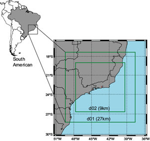
Atmospheric phenomena over the metropolitan area of Rio de Janeiro (Figure 1) are mainly related to the presence of the South Atlantic Convergence Zone (SACZ) (Ferreira et al., 2004; Seluchi and Chou, 2009), frontal systems (Seluchi and Chou, 2009; Dereczynski et al., 2009) or isolated convective systems (Britto et al., 2016). Figure 1S shows land use (top) and digital elevation model (bottom) of the metropolitan area of Rio de Janeiro (MARJ). Especially during the warm season, the proximity of Atlantic Ocean and different types of land use creates low-level atmospheric instability as a consequence of solar heating and evapotranspiration. The mountainous area of MARJ acts as a dynamic trigger for cloud development, which may lead to the occurrence of high rainfall accumulations, and local natural hazards such as floods and landslides (Roe et al., 2003; Barros et al., 2004; Boers et al., 2015; Oakley et al., 2017, Silva et al., 2016; Dereczynski et al., 2017).
To explore the local vertical profiles over different atmospheric scenarios in Rio de Janeiro a set of radiosondes RS92-SGP (http://www.vaisala.com) was used as a part of infrastructure provided by the Water Resources and Environmental Studies Laboratory (LABH2O/COPPE) of the Federal University of Rio de Janeiro (UFRJ). The atmospheric profiling data were collected outside of standard hours at 00:00 UTC and 12:00 UTC, between 11-November-2016 and 03-March-2018, corresponding to the warm and rainy season over the region (Dereczynski et al., 2009; Silva et al., 2017).
The methodology followed Silva et al. (2017), with additional radiosondes launched from the experimental site whenever a rainfall forecast was issued for the metropolitan area of Rio de Janeiro, for a total of thirty days and seventy radiosondes. Figure 2S shows the location of the site at the UFRJ campus. Radiosonde calibration followed the user’s guide manual available at the Vaisala website. Addition information on the accuracy of the measured parameters by Vaisala radiosonde sensors can be found in publications of the World Meteorological Organization (https://www.wmo.int/pages/prog/www/IMOP/publications/).
2.2 Cloud classification criteria
Radar reflectivity was used to diagnose and classify cloud types (Hagen et al., 2000; Punkka and Bister, 2005; Goudenhoofdt and Delobbe, 2013; Yang et al., 2013). Convective clouds are characterized by reflectivity echoes greater than 40 dBZ, while stratiform clouds present reflectivity between 20 dBZ and 40 dBZ and so-called nonprecipitating clouds present values lower than 20 dBZ (Hagen et al., 2000; Goudenhoofdt and Delobbe, 2013; Yang et al., 2013). According to these criteria, reflectivity data from the Sumaré weather radar (provided by the Alerta Rio system, http://alertario.rio.rj.gov.br/) was used to classify the days of the experiments. Table I shows the selected days according to the radar reflectivity criteria of clouds classification.
Table I Radiosonde experiments and cloud type classification
| Days with Radiosonde launches | Cloud type classification |
| 11/17/2016, 12/12/2016, 01/02/2017, 01/03/2017, 01/06/2017, 01/12/2017, 01/19/2017, 03/06/2017, 03/13/2017, 03/24/2017, 01/03/2018, 01/11/2018, 01/12/2018, 01/22/2018, 01/25/2018, 02/22/2018, 03/01/2018, 03/02/2018, 03/03/2018 | Convective |
| 11/18/2016, 01/13/2018, 01/15/2018, 03/08/2018 | Stratiform |
| 11/29/2016, 02/13/2017, 01/16/2018, 01/17/2018, 01/23/2018, 03/15/2018, 03/16/2018 | Nonprecipitating |
We selected three days for initial discussion during which these cloud types were observed over the study region: 02/22/2018, characterized by convective clouds (Figure 3S); 03/08/2018, characterized by stratiform clouds (Figure 4S); and 03/15/2018, characterized by nonprecipitating clouds. These days were also selected since they had the same number of radiosondes launched at the same hours, i.e., 15 UTC (12 Local Time (LT)), 17 UTC (14 LT), 19 UTC (16 LT) and 21 UTC (18 LT). Subsequently, the results considering all the selected days presented in Table I are also discussed.
2.3 Thermodynamic parameters and numerical modeling
Thermodynamic variables are utilized to evaluate atmospheric thermal parameters (temperature and moisture), especially as those relate to the convective cloud environment (Teixeira and Satyamurty, 2007; Busuioc et al., 2015). Dynamic variables characterize atmospheric motions (both wind speed and direction) and are generally dependent on large-scale and local circulation patterns (Rudolph and Friedrich, 2014). Simultaneous presence of these thermodynamic and dynamic parameters on a given time of day, cloud formation is expected to take place within the expected horizon (Wetzel and Martin, 2000; Nascimento, 2005; Silva et al., 2017).
Given the days selected according to the criteria of clouds classification, this work sought to analyze and compare the behavior of thermodynamic and dynamic variables for days categorized as having convective, stratiform and nonprecipitating clouds. Table II presents the thermodynamic and dynamic parameters chosen for this study: convective available potential energy (CAPE), convective inhibition (CIN), lifted index (LI), K index (K), Total Totals (TT) index, environmental lapse-rate (LR), velocity convergence (CONV), velocity divergence (DIV), wind shear (WS) and vertical movement (MV). Variables related to the state of the atmosphere were also chosen. Those include surface air temperature (TEMP), surface dewpoint temperature (DEWT), surface air depression (DEP) and precipitable water (PW).
Table II Thermodynamic and dynamic parameters
| Variable | Formula |
| Air depression |
|
| Convective potential available energy |
|
| Convective inhibition |
|
| Lifted index |
|
| Lapse-rate |
|
| K index |
|
| TT index |
|
| Precipitable water |
|
| Velocity convergence |
|
| Velocity divergence |
|
| Wind shear |
|
| Vertical motion |
|
In the formulas of the variables presented in Table II, T and Td represent air and dewpoint temperatures (measured in degrees centigrade (ºC)), respectively, while the subscripts refer to surface (SFC) or isobaric levels (hPa). Tp expresses the temperature of a lifted parcel (using the parcel method) at 500 hPa; Tvp and Tv (also in ºC) characterize the virtual temperature of a lifted parcel and the surrounding environment temperature, respectively. LFC represents the level of free convection (i.e. lifted parcel is warmer than surrounding environment), while LNB represents the neutral buoyancy level. The physical interpretations of the variables in Table II are briefly described below.
Surface air depression represents the difference between air temperature (TSFC) and dewpoint temperature (TdSFC), an indicator of moisture availability in the atmosphere. Convective available potential energy (CAPE) represents the energy of an air parcel calculated as the difference between parcel virtual temperature (Tvp (z)) and environment virtual temperature (Tv(z)) from LFC until LNB (Blanchard, 1988). Conversely, convective inhibition (CIN) is related to the energy (work) required to lift the air parcel from surface (SFC) to the LFC. Graphically, CAPE represents a “positive area” and CIN a “negative area” in the Skew T log P diagrams. The lifted index (LI), measured by the difference between the T of a lifted parcel (Tv500) and the surrounding air (Tv500) at 500 hPa (Galway, 1956), graphically expresses the “width” measurement of CAPE.
The lapse-rate (LR) represents temperature variation for an atmospheric layer. Typically, the layer between 700 hPa and 500 hPa is also a measurement of CAPE “width” (Nascimento, 2005), which we will adopt in this study. The K index represents the sum of air and dew point temperatures measured at 850 hPa subtracted from air depression at 700 hPa and air temperature at 500 hPa (George, 1960). The Total Totals index (TT) is quite similar to the K index, with the main difference being that air depression at 700 hPa is not considered in the calculation of TT (Miller, 1972). If the atmosphere is vertically warm and wet, K and TT present similar behavior. In contrast, in case a dry layer is present at 700 hPa, TT is not affected and can better represent atmospheric instability (Silva Dias, 1987; Henry, 1999; Nascimento, 2005). Precipitable water (PW) represents the available rain water if all water vapor integrated over an atmospheric column (this study integrated from surface to 100 hPa) precipitated (Silva et al.,2018).
To analyze the behavior of thermodynamic parameters during the classified days (Table I), upper air sounding data was plotted in SkewT/LogP diagrams using the SkewT 1.1.0 Python software package (https://pypi.python.org/pypi/SkewT) and the MetPy Python package (https://pypi.org/project/met/) was used to calculate the thermodynamic parameters.
The dynamic parameters were calculated using Weather Research and Forecasting (WRF) model (Skamarock et al., 2008) version 3.8. The model was configured with two nested domains, with horizontal spatial domain resolutions for coarse grid (d01) and fine grid (d02) of 27 km and 9 km, respectively, 27 vertical levels with the highest level at 50 hPa, and 4 vertical levels of soil. The green squares in the Figure 1 show the horizontal domains used. The physical parameterizations selected were: the WRF single-moment 3-class microphysics scheme (Hong et al., 2004), the Kain-Fritsch cumulus parameterization scheme (Kain 2004), the Rapid Radiative Transfer Model for longwave radiation (Mlawer et al., 1997), the Dudhia shortwave radiation scheme (Dudhia, 1989), the Unified Noah land surface model (Tewari et al., 2004), the Revised MM5 Monin-Obukov (Jiménez et al., 2012) for surface layer, and the Yon-Sei University Planetary Boundary Layer parameterization scheme (Hong et al., 2006). Initial and lateral boundary conditions were obtained from the Global Forecast System (GFS, http://www.emc.ncep.noaa.gov/GFS/doc.php) at six-hour intervals and horizontal resolution of 0.50º x 0.50º and provided to the WRF model.
Horizontal negative velocity convergence (CONV) and divergence (DIV) are essential dynamic and trigger mechanisms to promote air motions throughout the atmosphere (Doswell, 1987; Tajbakhsh et al., 2012; Silva et al., 2019). Given these distinct mechanisms related to convective and stratiform clouds (Homeyer et al., 2014), this study considered the atmospheric levels between 1000 hPa and 850 hPa to characterize convergence (CLL) and divergence (DLL) in the lower troposphere, the layer between 700 hPa and 500 hPa to characterize CONV (CML) and DIV (DML) in the middle of the atmosphere, and the atmospheric level from 300 hPa to 200 hPa to characterize upper CONV (CUL) and DIV (DUL). Wind shear (WS) was calculated as the difference between wind speed and direction in two atmospheric levels (at 10 meters and 500 hPa). Vertical motion (MV) at 500 hPa is also a dynamic trigger for cloud development, where positive values characterize upward motion (Houze,1993; Banacos and Schultz, 2005; Chen et al., 2006; Baba, 2016).
3. Results and Discussion
3.1 Case studies
Analysis of upper air sounding data and the SkewT/LogP diagrams made it possible to verify the atmospheric vertical profile through measurements of air temperature (red line) and dew point temperature (blue line) for 15 UTC (12 LT), 17 UTC (14 LT), 19 UTC (16 LT), 21 UTC (18 LT) on February 22 (Figure 1), March 8 (Figure 2) and March 15 (Figure 3), 2018. The circles filled in red and gray represents the LFC and LNB, respectively. For all days, small rates (~5.7 ºC km-1) of air temperature decrease throughout the troposphere are observed. This vertical profile is related to coastal regions, in this case to the proximity of the study region to the Atlantic Ocean, which tends to exhibit lower vertical air temperature profile rates compared to interior continental regions (Holton et al., 2002).

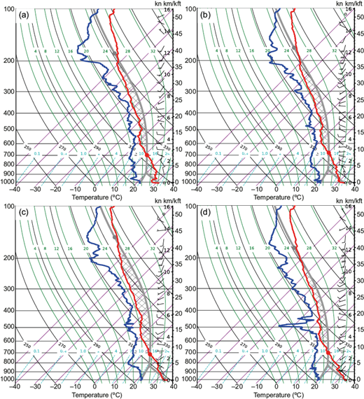
Fig. 2 SkewT/LogP diagram at: (a) 15 UTC, (b) 17 UTC, (c) 19 UTC and (d) 21 UTC on February 22, 2018.

On February 22 late morning (Figure 2a), a near-saturated (moisture availability) unstable-temperature atmospheric layer is observed from surface to 600 hPa; a dry layer is observed from 600 hPa to the upper atmospheric levels. In early afternoon (Figure 2b) and mid-afternoon (Figure 2c), a progressive increase of moisture is observed from surface to upper levels. Large potential energy (gray shaded area on SkewT/logP diagram) is observed in all soundings on this day, driving an air parcel ascending vertically from the LFC to the LNB (Figure 2) with CAPE values reaching above 3000 J.Kg-1 (Houze, 1993; Schultz et al., 2000). This potential energy was mainly related to the presence of the South American Convergence Zone (SACZ), which configures the northwest flow and brings warmer and moister air from the Amazon region towards the metropolitan area of Rio de Janeiro (Ferreira et al., 2004; Quadro et al., 2012), where lower atmospheric levels show local instability from solar heating and evapotranspiration near the surface during warm season (Doswell, 2001). Figures 5S and 6S show the corresponding satellite image and surface charts provided by the Center for Weather Forecasting and Climate Studies (http://satelite.cptec.inpe.br/home/index.jsp), indicating the SACZ configuration over South America. In addition, the SACZ also provides a dynamic environment favorable for upward air motion, reinforcing the deep convection observed in Figure 3S (Mota and Nobre, 2006; Tavares and Mota, 2012; Gille and Mota, 2014).
A similar vertical profile of moisture is observed on March 03, 2018 compared to February 22. However, for all sub-daily soundings launched on March 03, a more saturated atmospheric layer is observed from surface to 550 hPa (Figure 3). We observed no significant potential energy (gray shaded area) during this day. Such condition indicates the importance of a dynamic mechanism in the development of stratiform clouds (Figure 4S) within a moisture content local cloud scale environment in the absence of significant CAPE (Doswell, 2001; Itterly et al., 2018).
On March 15, the SkewT/logP diagrams (Figure 4) show CAPE and an unstable temperature profile, which corroborates the warm season daily cycle of solar heating warming the troposphere by conduction of atmospheric layer closest to the surface and subsequent convection (Seidel et al., 2005). However, in contrast to February 22 and March 03, significan CIN (beige area in the SkewT/Log P diagrams) is observed, requiring the need for dynamic forcing in order to develop clouds (Doswell, 2001).
CAPE, CIN, Lapse-Rate (LR), and LI, K and TT indices were calculated from the upper air sounding data to evaluate and intercompare sub-daily (15 UTC, 17 UTC, 19 UTC and 21 UTC) thermodynamic variations related to the three cloud types categorized, i.e., convective on February 22 (Figure 3S), stratiform on March 8 (Figure 4S) and nonprecipitating on March 15, 2018. The results are shown in Figure 5, where the convective day is represented by “Conv”, stratiform day is represented by “Strat” and nonprecipitating day is represented by “NoRain”.
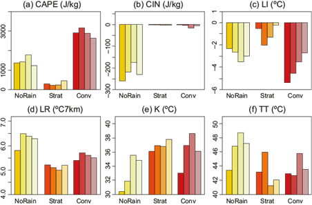
Fig. 5 Sub-daily (15 UTC, 17 UTC, 19 UTC and 21 UTC) variations of thermodynamic indices: (a) - CAPE; (b) - CIN; (c) - LI; (d) - K ; (e) - TT and (f) - LR on March 15 (“NoRain”), March 8 (“Strat”) and February 22 (“Conv”) 2018.
Significant CAPE (above 2500 J.Kg-1) values are observed for the convective day (Figure 4a), while non-significant CAPE values are observed for the stratiform day (Figure 4b), as seen in the Skew T Log P diagrams (Figure 3). Despite the intermediary CAPE values on March 15, it is possible to observe the presence of CIN (Figure 5b) with values between -100 J.Kg-1 and -300 J.Kg-1, which were not observed on February 22 (Figure 5b) and March 8 (Figure 5b). The LI index (Figure 5c) also shows its largest values (below -5 ºC) only on the convective day, characterized by the larger broad area observed in the SkewT/logP diagrams (Figure 2), corroborating the presence of atmospheric thermodynamic potential energy driving development of the convective clouds observed on this day (Nascimento, 2005; DeRubertis, 2006). In the opposite direction of CAPE behavior, LR sub-daily variations (Figure 5d) present significant values (above 6.5 ºC km-1) only during the nonprecipitating day (Figure 5d). This suggests that smaller moisture availability in the atmospheric lower levels could be producing warm air lifting following the adiabatic curve in the SkewT/logP diagrams (Figure 4) and, consequently, higher levels of air saturation (higher CIN). K (Figure 5e) and TT (Figure 5f) presented values above 30 ºC, as well as 40 ºC, for the three days analyzed, which indicate high storm potential with likely intense rainfall (Nascimento, 2005). This behavior was observed because these two indices are not able to represent atmospheric instability if it occurs below the 850 hPa threshold, suggesting that the main thermodynamic characteristics over the analyzed region are observed in the atmospheric layer closest to the surface (DeRubertis, 2006; Silva et al., 2017).
Figures 6 and 7 present WRF simulations for: on the left column, air temperature at 2 m and wind circulation at 850 hPa (T2M+WD); on the middle column, wind convergence (negative shaded area) and divergence (positive shaded area) at 1000 hPa and wind convergence (negative lines) and divergence (positive lines) at 850 hPa (CV+DV); and on the right column, wind shear between 500 hPa and 10 meters and wind convergence (negative lines) and divergence (positive lines) at 250 hPa (WSH + DVM) for 15 UTC (Figure 6) and 17 UTC (Figure 7) on February 22 (top row), March 8 (middle row) and March 15 (bottom row), respectively.

Fig. 6 WRF simulations for: on the left column, air temperature at 2 m and wind circulation at 850 hPa (left); on the middle column, wind convergence (negative shaded area) and divergence (positive shaded area) at 1000 hPa; convergence (negative lines) and divergence (positive lines) at 850 hPa (middle); and on the right column, wind shear between winds at 500 hPa and 10 meters; and convergence (negative lines) and divergence (positive lines) at 250 hPa at 15 UTC on February 22 (top row), March 8 (middle row) and March 15 (bottom row).
On February 22, wind circulation at 850 hPa shows a northwest flow advecting moist and warm air from the Amazon region towards the metropolitan area of Rio de Janeiro (Figure 6a) and the adjacent Atlantic Ocean (Figure 7a) at 15 UTC and 17 UTC. Such atmospheric pattern is related to the configuration of SACZ (Teixeira and Satyamurty, 2007). It is possible to observe a coupling between convergence (negative lines over negative areas) in the lower atmospheric levels (Figure 6b and 7b) and divergence at the upper levels (Figures 6c and 7c). This behavior shows an atmospheric vertical structure promoting a dynamic mechanism to lift air parcels and develop convective clouds (Doswell, 1987; Tajbakhsh et al., 2012). Weak wind shear is also observed, which can create an atmospheric environment to develop heavy rainfall (Silva et al., 2017).
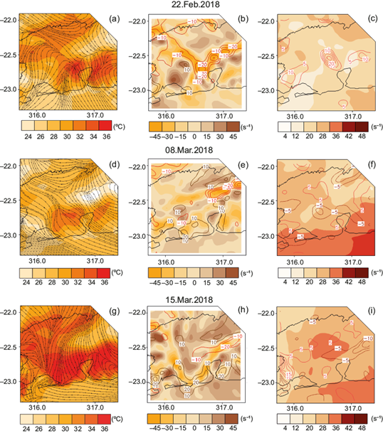
A different pattern is observed on March 8 at 15 UTC (Figure 6, middle row) and 17 UTC (Figure 7, middle row), with 850 hPa wind circulations indicating a southeast flow advecting moist air from the Atlantic Ocean (Figure 6d). This atmospheric circulation was related to a high-pressure system which brought cold air from higher latitudes towards the metropolitan area of Rio de Janeiro (Bonnet et al., 2018). Wind convergence at 1000 hPa (Figure 6e) was aligned under a wind divergence at 850 hPa (Figure 6e); suggesting upward vertical motion confined within this layer. At upper levels, wind convergence (Figure 6f and 7f) can also be observed. These occurrences of simultaneous wind convergence and divergence throughout lower and upper levels characterize the physical structure of stratiform clouds, i.e. a shallow and layered configuration, consistent with the results found by Collier (2006).
On March 15, the pattern of convergence and divergence at lower (Figures 6h and 7h) and upper layers (Figures 6i and 7i) is similar to March 8. The main difference was observed for wind circulation at 850 hPa, which showed a northeast component over Rio de Janeiro city. As a consequence, this scenario promoted a decrease of moisture and thermodynamic availability favoring cloud formation but without the potential for droplet growth and precipitation (Moraes et al., 2005; Moura et al., 2013).
The simultaneous presence of atmospheric instability and moisture is an important condition for convective clouds, observed by the high values of CAPE, LI, K and TT convective days (Figure 5). Vertical dynamic coupling is seen by means of the wind convergence at low level and divergence at upper levels. Over the metropolitan area of Rio de Janeiro, stratiform days are observed mainly after the passage of cold fronts and the presence of the migratory high pressure system with advection of cold air and moisture at low levels (Bonnet et al., 2018). This local pattern corroborated the lower LR values (Figure 5d) and the divergence behavior analyzed (Figures 6 and 7). On days with non-precipitating clouds, despite the presence of thermodynamic instability, higher CIN values (Figure 5b) and wind divergence at low levels were observed, suggesting the absence of dynamic triggers for ascent and clouds with precipitation development. These initial results indicate that analyses associated with the behavior of dynamic and thermodynamic variables under different atmospheric scenarios can provide qualitative tools for local predictors and warning systems, especially in the face of severe weather events.
3.2 Statistical overview
In order to describe qualitative and quantitative analyses related to the atmospheric environment of convective, stratiform and nonprecipitating clouds during the experiments made by LABH2O between 11-November-2016 and 03-March-2018, statistical analyses were conducted of vertical atmospheric profiles, wind, and thermodynamic and dynamic parameters. It is important to note that results may have some implicit biases due to the short period considered. As such, the main goal of these analyses is not to establish quantitative thresholds, but rather to characterize differences regarding the cloud types categorized.
Figures 8-10 illustrate the mean profile for the selected days presented in Table I. Qualitatively, a greater average CAPE (gray hatched area) can be observed on convective cloud days (Figure 8), possibly related to the simultaneous presence of warming and moisture content at low (1000-850 hPa) level. The mean profile for stratiform (Figure 9) and nonprecipitating (Figure 10) cloud days presented less CAPE than convective days (Figure 8). The stratiform days (Figure 9) presented more moisture availability, between 1000-600 hPa. However, there is a lower surface mean temperature (~27 ºC) compared to convective days (~31 ºC) suggesting the importance surface warming for convective development. Nonprecipitating days (Figure 10) presented the highest surface mean temperature (~33 ºC), but also the largest CIN area (yellow hatched area) and a dry layer between1000-900 hPa.
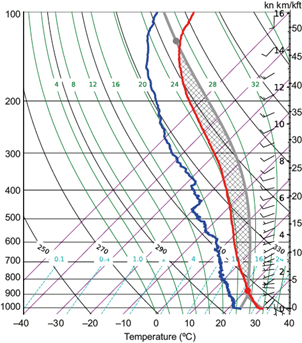


Fig. 10 SkewT/LogP mean diagram for the nonprecipitating cloud days between November 2016 and March 2018.
Figure 11 shows thermodynamic variables and dynamic variable boxplots for convective (red), stratiform (orange) and nonprecipitating (yellow) cloud days. The thermodynamic parameters (Figure 11a to 11l) were calculated using the upper air sounding data collected during the experiments. The dynamic parameters were calculated using the results of the WRF numerical model. Given the spatial diversity of wind convergence and wind divergence, a region surrounding the campus of Federal University of Rio de Janeiro (UFRJ) was used to evaluate the local effects of this trigger during the thirty days (Table I).

Fig. 11 Boxplots of thermodynamic and dynamic variables for the convective (red), stratiform (orange) and nonprecipitating cloud days (yellow) between November 2016 and March 2018.
The higher temperature (~33 ºC) and lower dew point temperature (~21 ºC) (Figure 11a and Figure 11b) were observed for the nonprecipitating cloud days. The stratiform cloud days presented the lower temperature (27 ºC) and dew point depression (2 ºC) (Figure 11a and 11c). The higher dew point temperature (23.5 ºC) was observed for the convective days (Figure 11b), since moisture is an important ingredient for convective cloud development (Doswell, 2010; Pucik et al., 2015). The combined presence of low-level higher moisture (Figures 11b and 11c) and diurnal warming (Figure 11a and Figure 11e) resulted in the highest CAPE (around 2600 J Kg-1) and low CIN (~-15 J Kg-1) on convective days (Figure 11d). Analyzing severe and nonsevere storms, Pucik et al. (2015) verified that CAPE values diminish for decreasing severe weather intensity, corroborating the results between the three categorized clouds.
LFC was highest (860 hPa, corresponding to lower altitude) on stratiform cloud days, followed by convective (820 hPa) and nonprecipitating (740 hPa) days (Figure 11f). The nonprecipitating cloud days presented high LFC (740 hPa) and LNB (165 hPa) values, indicative of the small layer with thermodynamic available energy. Convective days were also characterized by the most negative LI values (-4 ºC) compared to the other days (Figure 11h), suggesting that besides the larger vertical extension of thermodynamic energy (Figures 11f and 11g), the atmosphere also tended to present a “greater width” with respect to this distribution of energy along the analyzed period (Nascimento, 2005; Tajbakhsh et al., 2012; Pucik et al., 2015).
The LR (Figure 11i) presented the highest values (6 ºC/km) for the nonprecipitating cloud days. As previously discussed, this could be a result of the higher temperatures values (Figure 11a) and the lowest moisture availability (Figure 11c), causing air parcels to ascend dry adiabatically and resulting in higher cooling rate through the vertical profile (Tajbakhsh et al., 2012). Convective and stratiform days, however, presented lower LR values (Figures 11b and 11c), which could be related to liberation of heat latent in the atmosphere due to higher moisture availability. On convective cloud days the results agree with the evaluation conducted by Taszarek et al. (2017) of sounding-derived parameters associated with convective hazards in Europe, in which the authors verified that convective cloud development occurred in environments with lower lapse rates, high CAPE and high low-level moisture. The K (Figure 11j) and TT (Figure 11k) indices presented significant K values (above 30 ºC) and TT above 40 ºC (Silva Dias, 2000) for the three cloud types, confirming the previous discussion presented in Figure 6 and the results found in DeRubertis (2006) and Silva et al. (2017). Higher PW values were observed for the convective (53 mm) and stratiform (56 mm) days, also agreeing with the results found for other moisture variables (Figures 11b and 11c).
Among the dynamic triggers, the CLL layer (Figure 11m) presented the most expressive convergence (negative) values in the convective days (-16.5 s-1). This characteristic, associated to the low-level moisture (Figures 11b and 11c) and thermodynamic instability (Figure 11d), could have created the atmospheric environment on convective days observed (Boer et al., 2013). An opposite behavior was observed for the DLL (Figure 11n) and DML (Figure 11p) layers with the highest (positive) values for the nonprecipitating days (9.7 s-1 and 7.3 s-1, respectively). CLL values (-11.7 s-1) in the stratiform days also could characterize the effects of air friction by changing surface wind flow from ocean to continent over the analyzed period (Bonnet et al., 2018). However, DLL (Figure 11n) and DML (Figure 11p) values (6.4 s-1 and 6.9 s-1, respectively) were observed on stratiform days. An opposite mechanism for CLL (Figure 11m) and DML (Figure 11p) suggested that air confinement between these layers was occurring on stratiform days. Consequently, cloud development under this atmospheric environment tended to present the shallow and layered development characteristic of stratiform clouds (Collier, 2006).
At upper levels, higher CUL values (Figure 11q) and lower DUL values (Figure 11r) were observed on stratiform (-4.5 s-1 and 3.2 s-1, respectively) and nonprecipitating (-4.4 s-1 and 2.8 s-1, respectively) days, corroborating the dynamic mechanism observed in the middle atmospheric levels for this type of clouds (Tajbakhsh et al.,2012). On convective days, however, we observed higher (negative) CLL and CML values (Figures 11m and 11o) (-16.5 s-1 and -9.6 s-1, respectively) under higher (positive) DUL values (Figures 11r) (8.3 s-1), which agrees with the mass conservation principle and suggests a dynamic vertical structure configuration for convective development (Clark et al., 2009; Silva et al., 2017). The highest wind shear (11.5 s-1) was observed during stratiform events (Figure 11s), while the largest vertical motion (0.3 m/s) was observed during convective events (Figure 11t). This is consistent with the results found by Silva et al. (2017), whereby weak wind shear and vertical motion could act as a dynamic trigger for convective clouds.
4. Conclusions
This study evaluated the thermodynamic and dynamic atmospheric conditions relying on upper air sounding data and numerical simulations as they relate to the formation of convective, stratiform, and nonprecipitating clouds over the metropolitan area of Rio de Janeiro (MARJ), Brazil. A radar echo reflectivity criterion was used to classify such cloud types. Three days (February 22, March 03 and March 15, 2018) were initially chosen as representative of each of the three cloud types to qualitatively analyze the dynamic and thermodynamic characteristics associated with them.
Significant potential energy (CAPE > 2500 JKg-1) was driving air parcels and vertical ascent on convective cloud day (February 22, 2018). The stratiform day (March 03, 2018) presented a similar vertical moisture profile, but no significant CAPE was available, suggesting the importance of dynamic mechanisms for stratiform clouds development within a moist local scale environment. The nonprecipitating day (March 15, 2018) showed potential energy and an unstable temperature profile. That being said, in contrast to convective and stratiform days, there is a need for external work for air parcel ascent on this day given CIN values between -100 J Kg-1 and -300 J Kg-1, requiring dynamic forcing to develop clouds.
The statistical overall evaluation and metrics calculated considered all the experimental days between November 2016 and March 2018. The results showed that the mean values of higher moisture (Td ~23.5 ºC) combined with the diurnal warming (31 ºC) would have resulted in the highest CAPE (~ 2600 J.Kg-1) and lowest CIN (around -15 J.Kg-1) observed on convective days. Nonprecipitating cloud days showed the highest temperature (~33 ºC) and lower moisture (Td ~ 21 ºC). Stratiform days presented the lowest temperature (27 ºC) and intermediate moisture (Td ~23 ºC).
Furthermore, convective days also presented the greatest negative LI values (-4 ºC), suggesting that besides the larger vertical extension of thermodynamic energy, the atmosphere also tended to present a “greater width” of the referred energy distribution in the atmosphere. The lapse rate was highest values (6 ºC/km) on nonprecipitating cloud days, a result of the higher temperature and the lower moisture availability, causing air parcels to ascend dry adiabatically and presenting a higher cooling rate through the vertical profile. K and TT presented significant values (> 30 ºC and 40 ºC) for the three cloud types, possibly as a result that these two indices are not able to represent atmospheric instability if it occurs below the 850 hPa level. Convective and stratiform days presented higher PW values (53 and 56 mm) suggesting the relevance of moisture availability for cloud development.
Regarding the dynamic triggers, convective days presented the most relevant low-level convergence and upper-level divergence (-16.5 s-1 and 8.3 s-1, respectively), which associated with low-level moisture and thermodynamic instability could have created the atmospheric environment for this cloud type. Indeed, such pattern agrees with mass conservation and characterizes the dynamic vertical structure and increased potential for convective development.
Stratiform days showed a different dynamic mechanism, with low-level convergence occurring under a mid-level divergence layer. In this case, such profile suggests vertical air confinement between those layers and horizontal spread creating an atmospheric environment favorable for shallow and layered clouds. Nonprecipitating days presented a similar behavior, but with a small moisture and thermodynamic availability. In general, results show a coupling of wind convergence, moisture and energy in the lower atmospheric levels and divergence in the upper atmospheric levels on convective days. Despite the moisture availability observed on stratiform days and the thermodynamic energy on nonprecipitating days, the respective coupling between these conditions and dynamic triggers was not observed.

