nueva página del texto (beta)
 Inglés (pdf)
 Artículo en XML
 Referencias del artículo
 Enviar artículo por email
 Citado por SciELO
  Similares en
SciELO
Similares en
SciELO 
 Permalink
1. Introduction
The influence of large-scale climate oscillations on hydrological variables affects the natural water supply of a specific region (Ouachani et al., 2013; Nalley et al., 2016). A leading pattern of weather and inter-annual climate variability over Colombia is El Niño Southern Oscillation (ENSO) (Poveda and Mesa,1997). ENSO results from the ocean-atmosphere interaction that causes positive and negative anomalies of the sea surface temperature (SST) in the central and eastern tropical Pacific. The warm phase is known as El Niño, and the cold phase as La Niña and its effects are not universal in their timing, sign, or magnitude (Tedeschi et al., 2015).
For the case of Colombia, several studies through linear correlation have shown that ENSO strongly influences its hydroclimatology. El Niño has been related to negative rainfall and streamflow anomalies and La Niña to the opposite behavior. The strongest relation occurs from December to February and the weakest from March to May. Studies have also shown that the impact of ENSO on hydrological variables propagates from west to east and that north and central regions experience the most significant impact, while east and southeast regions are less affected (Poveda et al., 1997; 2006; 2011; Córdoba-Machado et al., 2015a; Córdoba-Machado et al., 2015b). El Niño is also associated with extreme events such as droughts, frosts, forest fires, and La Niña with torrential rains, floods, and landslides (Hoyos et al., 2013; Córdoba-Machado et al., 2015a). One of the most serious consequences of ENSO events is the shortage of drinking water, which causes human health problems and affects food production.
Although linear correlation methods revealed the connection between ENSO and climate variables, the linear coefficients obtained are usually low, a fact that requires the use of other methodologies such as spectral analysis to explore more characteristics of each of the series and its relationship with another series (Fu et al., 2012; Jiang et al., 2019).
Several studies have explored spectral analysis based on Fourier Transform (FT), Wavelet Transform (WT), or Hilbert-Huang transform (HHT), to improve knowledge of climate variability in Colombia at different time scales. For example, Poveda et al. (2002a) used FT and WT and found that El Niño diminished the diurnal rainfall cycle while La Niña intensifies it. Poveda et al. (2002b) implemented WT to identify changes in average monthly river flow during warm events. Arias and Poveda (2005) studied the space-time variability of rainfall in Colombia through Empirical Orthogonal Functions (EOF) and WT for monthly records; they found that the first EOF explains 90% of the variance associated with annual and semi-annual periodicities resulting from the meridional oscillation of the Intertropical Convergence Zone (ITCZ). The WT of this first EOF exhibits significant variance at 4-8 months and 8-16 months, whose relative importance varies with time. Rueda and Poveda (2006) found a significant coupling between ENSO and the annual advection cycle of low-level winds known as “Chocó Jet.” Carmona and Poveda (2012 and 2014) explored FT, WC, and HHT to detect principal modes of hydroclimatic variability in Colombia; they also identified links between ENSO and precipitation, temperature, and river discharge. More recently, Restrepo et al. (2019) implemented HHT and WT to identify the contribution of low-frequency climatic-oceanic oscillations to streamflow variability in coastal rivers of the Sierra Nevada de Santa Marta (Colombia). All these studies have detected evidence of the ENSO-precipitation relation; however, they have also established that ENSO teleconnections have substantial heterogeneity at different spatio-temporal scales over Colombia. This heterogeneity has been attributed to several factors, such as the country’s orography, geographical aspects like the proximity to the Pacific Ocean, the Caribbean Sea, and Amazonia. More specifically, links to the dynamics of the three main low-level jets (LLJ), the Caribbean LLJ, the Chocó LLJ, and Orinoco LLJ, and also the Cross-Equatorial Flow (CEF). All of them co-occur and mutually influence one another, generating moisture advection anomalies during ENSO phases that are different for each region of the country (Poveda et al., 1997, 2006, Salas et al., 2020). Therefore, there is still a need to carry out studies to determine local ENSO influences in more detail (Sun et al., 2017; Restrepo et al., 2019).
Another method used to assess links between large-scale climate oscillations and local climate variability is coherence analysis (CA). CA applied the idea of time-varying coherence using time-frequency analysis methods like FT, HHT, or WT (Torrence and Compo, 2011; Massei and Fournier, 2012; Schulte et al., 2016; Restrepo et al., 2019). The Wavelet-based coherence (WC) and the HHT coherence (HHTC) are the most widely used time-varying coherence methods (Restrepo et al., 2019). WC was selected because previous results have shown that even though HHTC has higher time resolution and frequency resolution than WC under ideal conditions, the WC is more stable; further, it has been implemented and explored for climate teleconnection analysis with a proven performance (Zhang et al., 2004; Ouachani et al., 2013; Araghi et al., 2016; Nalley et al., 2016; Schulte et al., 2016, Restrepo et al., 2019).
WC can be used to identify the influence of large-scale climate indices on hydroclimatic variables in different regions. For example, Ouachani et al. (2013) applied WC to examine ENSO’s influence on precipitation and streamflow variability in the Mediterranean region. Kenner et al. (2010), and Sharma and Srivastava (2016) analyzed the same variables for southeastern United States. Fu et al. (2012) and Nalley et al. (2016) implemented WC to analyze the combined influence of solar activity and other dominant large-scale oscillations on streamflow across southern Canada, and Araghi et al. (2016) utilized WC to study the influence of ENSO on precipitation variability in Iran. More recently WC has also been implemented to assess extreme precipitation events and their spatiotemporal variability (Jiang et al., 2019), to study the simultaneous influence of climate teleconnections at differing time-frequency scales on precipitation and streamflow (Nalley et al., 2019; Das et al., 2020).
Studies provide evidence of ENSO’s influence on hydroclimatic variables in Colombia; the purpose now is to know in greater detail the nonlinear dynamics of this relationship and to improve forecasts, particularly in zones where impacts are significant and imply economic and life losses. Data from the Unidad Nacional para la Gestión del Riesgo de Desastres (National Unit for Disaster Risk Management -UNGRD) indicate that the economic losses of the last strong La Niña event (2010-2011) reached 6500 million dollars, equivalent to 5.7% of the gross domestic product during that time, and that an El Niño event of low to moderate intensity would cost more than 288 million dollars. The latest Estudio Nacional del Agua (National Water Study -ENA) also identified zones with increased risk of water shortage associated with climate variability (ENA 2018); between 300,000 and 500,000 people affected in those zones during El Niño 2015-2016 (UNGRD, 2016).
Moreover, around 70 % of the electric energy in Colombia is generated by hydropower plants, which depend on precipitation. Studies by Marengo and Espinoza, 2016 and Weng et al. (2020) indicate how El Niño linked with other anthropogenic causes, like deforestation, have magnified droughts and reduced river flows resulting in an energy crisis (Weng et al., 2020; Alves et al., 2017; Erfanian et al., 2017). For example, the 2015−2016 drought exceeded the severity of those associated with strong El Niño events 1982/1983 and 1997/1998 (Jiménez-Muñoz et al., 2016; Marengo et al., 2016). Research to understand these teleconnections can contribute to better energy planning. The methodology can also be applied to study other variables that support energy transition towards sustainability under climate change, offering security in the power supply.
Based on all the previous studies, the present paper evaluates nonlinear correlations of the ENSO-precipitation relationship, mainly over six regions where freshwater resources have been significantly reduced during the last El Niño events. Moreover, an attempt is made to identify which indices will enable improved predictability of hydroclimatological variables.
2. Methodology
2.1. Study area
The study area are six places in Colombia were the freshwater resources have been significantly reduced during the last El Niño events. Figure 1 displays the stations’ location. Wavelet transform (WT) and the wavelet coherence (CW) was performed with data from the indices that represent the ENSO and with monthly precipitation series for the period 1981-2016.

2.2. ENSO Data
Nine climate indices were selected to represent ENSO and obtained from the National Oceanic and Atmospheric Administration (NOAA) Climate Prediction Center (CPC) and the NOAA Earth System Research Laboratory’s Physical Sciences Division (PSD). The indices were Niño 1+2, Niño 3, Niño 3.4, Niño 4, ONI, SOI, BEST, ESPI, MEI. Table I presents a short description of these indices; a more detailed explanation of each index can be found in https://www.esrl.noaa.gov/psd/data/climateindices/list/.
Table I Indices used to represent ENSO
| Niño 1+2 | Extreme Eastern Tropical Pacific SST *(0-10S, 90W-80W). Data from CPC. |
| Niño 3 | Eastern Tropical Pacific SST (5N-5S,150W-90W). Data from CPC. |
| Niño 3.4 | East Central Tropical Pacific SST* (5N-5S)(170-120W). Data from CPC. |
| Niño 4 | Central Tropical Pacific SST *(5N-5S) (160E-150W). Data from CPC. |
| ONI | Oceanic El Niño Index calculated as the three-month running mean of SST anomalies in the Niño 3.4 region. Climatology used for the anomaly was 1986-2015. Data from CPC. |
| SOI | Southern Oscillation Index calculated as the pressure difference between Tahiti and Darwin. Data from CPC. |
| BEST | Bivariate ENSO Timeseries Calculated from combining a standardized SOI and a standardized Niño 3.4 SST timeseries. The values are averaged for each month and then, 3-month running mean is applied to both time series. Data from PSD. |
| ESPI | ENSO precipitation index estimates the gradient of rainfall anomalies across the Pacific basin and ensures a good relationship with SST- and pressure-based indices. Data from Curtis and Adler (2000). |
| MEI | Multivariate ENSO Index Version 2, MEI is the time series of the leading combined Empirical Orthogonal Function (EOF) of five different variables (sea level pressure (SLP), sea surface temperature (SST), zonal and meridional components of the surface wind, and outgoing longwave radiation (OLR)) over the tropical Pacific basin (30 ºS-30 ºN and 100 ºE-70 ºW). Data from PSD. |
The precipitation data were taken from two databases to compare results, the first from the Institute of Hydrology, Meteorology and Environmental Studies (IDEAM), and the second from the Climate Hazards Group InfraRed Precipitation (CHIRPS), which combines satellite with station data.
2.3. IDEAM Data
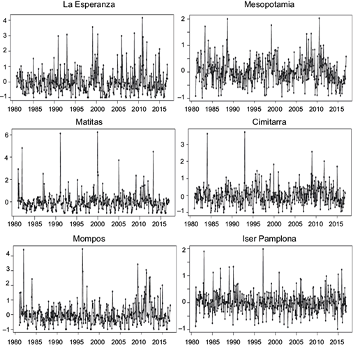
The Institute of Hydrology, Meteorology and Environmental Studies of Colombia (IDEAM) supplied the time series used for first analysis. This information corresponds to monthly precipitation series from six stations where there is a high probability of shortage during El Niño events (ENA 2019). Table II presents the rainfall stations’ characteristics and Figures 2 and 3 show the time series used. Figure 2 also presents the ENSO events with the most signifi cant consequences registered, red box for El Niño, and blue for La Niña episodes. Figure 3 presents the series of standardized anomalies for each station, which were calculated by dividing anomalies by the climatological standard deviation, and anomalies were determined by subtracting climatological values from data. Figure 3 provides more information about the magnitude of the anomalies without the influence of dispersion and helps to identify variability in recent years.
Table II Rainfall stations characteristics (Data from IDEAM)
| Station Name | Region | Longitude (º) | Latitude (º) | Altitude (m) | Mean annual rainfall (mm) | Standard Deviation (mm) | Coefficient of variation |
| La Esperanza | Caribe | -74,30 | 10,74 | 25 | 1378 | 921.88 | 0.67 |
| Matitas | Sierra Nevada de Santa Marta | -73,03 | 11,26 | 20 | 1171 | 468 | 0.39 |
| Mompós | Sinú San Jorge-Nechi | -74,43 | 9,26 | 20 | 1461 | 361 | 0.24 |
| Mesopotamia | Cuenca del alto Cauca | -75,31 | 5,88 | 2314 | 3445 | 651 | 0.19 |
| Cimitarra | Cuenca Medio Cauca y Alto Nechi | -73,95 | 6,30 | 300 | 2805 | 671 | 0.24 |
| Iser Pamplona | Cuenca del Catatumbo | -72,64 | 7,37 | 2340 | 925 | 243 | 0.26 |
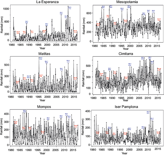
Fig. 2 Time series of the mean monthly rainfall data from IDEAM. The graphs indicate El Niño and La Niña events that have most affected precipitation levels. Red box for El Niño, and blue for La Niña episodes.
The methodology to calculate the anomalies can affect the results, as mentioned by Salas et al. (2020). However, other methods for calculating anomalies such as the F-filtering of the annual cycle by moving average, the annual cycle extracted by the singular spectrum, were explored, and the spectra obtained were not pretty different. However, this affirmation is qualitative and could be contrasted with a sensitivity analysis in further work.
2.4 CHIRPS Data
The U.S. Geological Survey (USGS) and the University of California, Santa Barbara (UCSB) created and supplied a public precipitation database called Climate Hazards Group InfraRed Precipitation (CHIRPS) available since 2014. CHIRPS data is available over land from 1981 to the present, with spatial resolution of 0.05º, from 50 ºS to 50 ºN for all longitudes. The temporal resolution provided is days, pentads, months, decades, and years. Monthly information was selected for the present case. CHIRPS was created with data from CHPClim (Climate Hazards Precipitation Climatology), Geostationary thermal infrared (IR), TRMM (Tropical Rainfall Measuring Mission, NOAA Climate Prediction System (CFSv2) atmospheric model of precipitation fields; and in situ observations of precipitation obtained from various meteorological services (Funk et al., 2015; Salas et al., 2020). In situ data for Colombia was provided by IDEAM and therefore, IDEAM and CHIRPS datasets are not so different, in fact CHIRPS has been validated for Colombia and this allows it to be use in places where there is no information (Urrea et al., 2016; Pedraza and Serna, 2018). The purpose of using both datasets (IDEAM and CHIRPS) is to compare whether the results obtained are similar and to verify if, for studies evaluating non-linear relationships, it may also be appropriate to use CHIRPS in those places without in-situ data. The precipitation time series from CHIRPS were taken from coordinates close to those of the six IDEAM stations. Table III presents the rainfall data from CHIRPS close to the in-situ stations, and Figures 4 y 5 show the time series anomalies created in the same way as with IDEAM data.
Table III Rainfall stations characteristics (Data from CHIRPS)
| Station Name | Region | Longitude (º) | Latitude (º) | Mean annual rainfall (mm) | Standard Deviation (mm) | Coefficient of variation |
| CHIRPS 1 | Caribe | -74,25 | 10,72 | 1095 | 200 | 0.18 |
| CHIRPS 2 | Sierra Nevada de Santa Marta | -73,1 | 11,32 | 994 | 326 | 0.34 |
| CHIRPS 3 | Sinú San Jorge-Nechi | -74,45 | 9,22 | 1452 | 325 | 0.22 |
| CHIRPS 4 | Cuenca del alto Cauca | -75,5 | 5,82 | 2376 | 378 | 0.16 |
| CHIRPS 5 | Cuenca Medio Cauca y Alto Nechi | -73,7 | 6,22 | 2933 | 252 | 0.085 |
| CHIRPS 6 | Cuenca del Catatumbo | -72,75 | 7,32 | 966 | 141 | 0.14 |
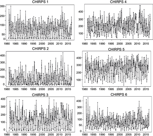
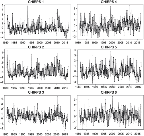
Tables II and III and Figures 2 to 5 show that although the coordinates used with both databases were as close as possible, there are several differences between them; for example, the values of the mean annual rainfall vary, the standard deviation, the coe- fficient of variation, as well as the number of highs and lows associated with El Niño or La Niña events, respectively. In general, in the selected stations, the CHIRPS series tend to present fewer local minima or maxima; this implies that ENSO’s influence may be more difficult to detect in these series, which is important to consider for this analysis.
2.5 Methods
2.5.1 Background of Wavelet transform (WT) computation
Continuous wavelet transform (WT) is a method to analyze the frequency and phase variations across time in a signal at several scales simultaneously (Torrence and Compo, 2011; Massei and Fournier, 2012; Schulte et al., 2016; Restrepo et al., 2019). The transform is defined as the convolution of the time series x t with a set of “daughter” wavelets Ψ (t - τ/s) which are generated by the “mother” wavelet Ψ(t) by translation in time by τ and scaling by s:
The symbol * represents the complex conjugate. The “mother” wave Ψ implemented in this case is a Morlet wavelet:
The angular frequency is set to six to make the Morlet wavelet approximately analytic; therefore, the period is 2π/6. The position of Ψ (t - τ/s) in the time domain is given by being shifted a dt. The value of s determines wavelet coverage of x t in the time-frequency (or time-scale) domain, the minimum (smín) and maximun (smax) scale are the minimum and maximum values of s respectively (Torrence and Compo, 2011; et al., 2016, 2019).
There are multiple options to select the mother wave however, previous research about the time-frequency evolutions of hydroclimatic series have shown that Morlet is better than others (e.g. Mexican Hat, Haar and others). The reasons for preferring Morlet are: 1. Frequency resolution is better; 2. Detection and localization of scale is improved; 3. Morlet detects peaks and valleys like the others and splits the wavelet into its real and imaginary parts. The real part describes oscillatory time series characteristics. The imaginary part conserves the phase information that is requisite when calculating the coherence wavelet with another time series, which is the main purpose of this work (Biswas and Si, 2011; Kravchenko et al., 2011).
The amplitude A of each periodic component found in x t and how it evolves with time is obtained by calculating:
This rectified version avoids the underestimate of high-frequency events. The square of the amplitude gives information about time-frequency wavelet energy density P x (τ, s) or wavelet power spectrum:
More detailed information of Eqns. (1) to (4) is presented in Torrence and Compo (2011), Nalley et al. (2016), and Restrepo et al. (2019).
The wavelet power spectrum is what allows the visualization of the frequency variation across time at different scales simultaneously. To calculate the wavelet transform it is necessary to consider the edge effect, which appears because the wavelet used to compute the CWT on non-cyclic data is not fully localized in time and frequency. Edge effects are overcome by padding the data with zeros; the prurpose is to complete the length of the time series up to the next scale. The edge effect is shown in the wavelet power spectrum as a concave-up shaped area called the cone of influence COI. The analysis of the wavelet transform power spectra must be limited to areas outside the COI.
The CWT also allows analyzing its phase changes. These variations in the displacements concerning a particular origin are given by the instantaneous wavelet phase, represented as:
Equation (5) is essential to study the nonlinear ENSO-precipitation relationship, which will be explored through the wavelet-based-coherence explained below.
2.5.2. Wavelet Coherence
The wavelet-based coherence (WC) is the method selected to compare the ENSO indices with the monthly precipitation time series. WC evaluates the frequency and phase synchronization among signals (Nalley et al., 2019; Das et al., 2020). WC is based on cross-wavelet analysis concepts; according to Veleda et al. (2012), the cross-wavelet transform is:
where T x (τ, s) and T y (τ, s) acording with equation (1), are:
The module of (6) is the cross-wavelet energy density and produces the cross-wavelet power spectrum useful to compare the two series:
The cross-wavelet is the covariance analog, but it depends on the unit of measurement of the series, defining wavelet coherency avoids an erroneous interpretation of the results (Torrence and Compo, 2011, Nalley et al., 2019; Das et al., 2020) and is defined as:
P x and P y are the wavelet power of each series defined as:
The letter s that precedes each amount indicates that these values should be smoothed. The wavelet coherency is an analogous concept to the classical correlation (Torrence and Compo, 2011, Nalley et al., 2019; Das et al., 2020); then, in this context the wavelet coherence is defined as the analogous to the correlation coefficient:
The value of the coefficient C2 x,y (x t , y t ) varies between 0 and 1, where 1 would indicate that the covariance between the series compared is maximum and 0 that there is no relationship.
To obtain information about the phase synchronization in terms of the instantaneous or local phase, we use the phase difference:
where ϕ x (τ,s) and ϕ y (τ,s), following Eqn. (5), are the individual phases of each signal. If phase difference has an absolute value less (greater) than π/2 it means that series move in phase (anti-phase), the sign of the phase difference indicates which signal leads the other.
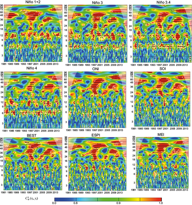
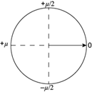
The wavelet coherence and phase difference results are displayed in a spectrum in a similar way to wavelet power spectrum. Here C 2 x,y (x t ,y t ) is represented by colors and ϕ x (τ, s) - ϕ y (τ, s) by arrows . An in-phase relationship is indicated by arrows that point straight to the right, and anti-phase relation is indicated by arrows pointing straight to the left. Other cases show a lead/lag relationship, when a ENSO index led the precipitation response (Nalley et al., 2016). Arrows are only plotted if C 2 x,y (x t ,y t ) >0.5, Table AI in Apendix A helps to better interpretate the direction of the arrows.
To interpret the phase difference between two signals, it helps to express the resulting angle, given in radians, in terms of units of time. The phase difference ϕ x (τ, s) - ϕ y (τ, s) varies between -π to +π; therefore, for a given period, the correspondence is made so that the duration of the entire period is equivalent to traversing all radians between -π to +π. For example, for a 12-month scale or period, a difference of phase of +π is equal to 6 months, one of +π/2 to 3 months; for a scale of 48 months, a phase difference of +π. would correspond to 24 months, one of +π/2 would be equivalent to 12 months and so on. Let us remember that the sign only refers to which signal is ahead of the other, as indicated in Table AI.
2.5.3. Statistical test of significance
The statistical significance was tested through simulation algorithms. The null hypothesis of “no periodicity” (for WT) or of “no joint periodicity” (for WC) can be assessed with a variety of alternatives to test against, for example, white or red noise, shuffling the time series, time series with a similar spectrum, AR, and ARIMA (Rösch and Schmidbauer, 2018). To determine the significance levels for wavelet spectra or wavelet coherence spectra it is necessary to choose a background spectrum to compare against. The theoretical white noise wavelet power spectra were chosen to derive and compare via Monte Carlo using 1000 simulations. A complete explanation is provided in Rösch and Schmidbauer (2018) and Torrence and Compo (2011).
All spectra obtained contain the cone of influence and contour lines that delimit the areas where results are statistically significant at the confidence interval > 95%, i.e., at 5% significance level.
The Waveletcomp library of R (Rösch and Schmidbauer, 2018) was used to compute the wavelet transforms and the coherence wavelet power spectra; Table AII in apendix A presents parameters used in the script.
2.6 Procedures
The wavelet coherence analysis, carried out with each database (IDEAM and CHIRPS), proceeded as follows:
The WT procedures were computed on monthly precipitation data from IDEAM to evaluate their time-frequency variability. Results are shown in Figure 6.
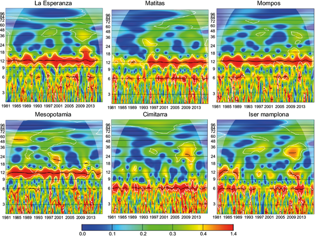
Fig. 6 Continuous wavelet spectra of the monthly precipitation data. Colors represent power P x (τ,s). The cone of influence is located outside of the lines with a concave-down shape, and the thick white lines enclose regions of significant periodicities at 5%. Data from IDEAM.
Step 1. is repeated but with the CHIRPS precipitation data. Results are shown in Figure 7.
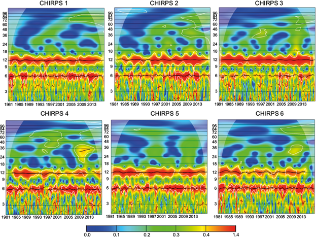
Fig 7 Continuous wavelet spectra of the monthly precipitation data. Colors represent power P x (τ,s). The cone of influence is located outside of the lines with a concave-down shape, and the thick white lines enclose regions of significant periodicities at 5%. Data from CHIRPS
The WT procedures were computed on ENSO indices to evaluate their time-frequency variability. Results are shown in Figure 8.
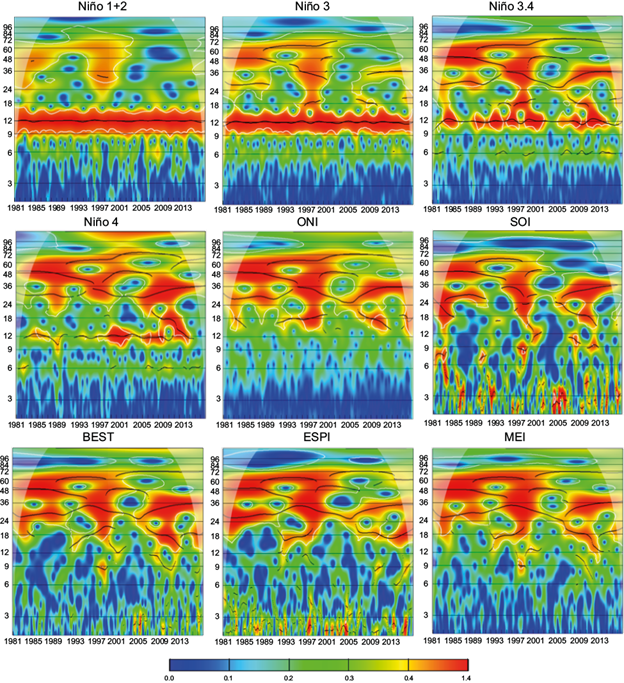
Fig 8 Continuous wavelet spectra of the ENSO indices. Colors represent power P x (τ,s). The cone of influence is located outside of the lines with a concave-down shape, and the thick white lines enclose regions of significant periodicities at 5%.
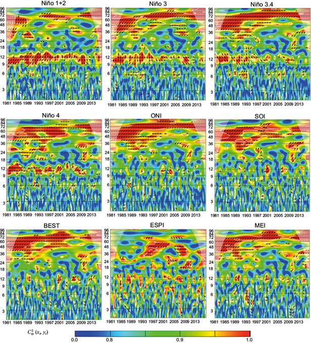
The WC procedures were computed between the monthly precipitation from IDEAM and indices: Niño 1+2, Niño 3, Niño 3.4 and Niño 4, i. e. the SST of these regions (Table I). Results are shown in the first four panels in Figures 9, 10, 11, 12, 13 and 14.
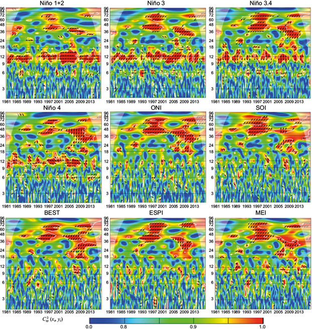
Fig 9 Wavelet coherence C 2 x,y (x t , y t ) and phase difference Arg (T x,y (τ,s)) between ENSO indices and precipitation of La esperanza station. The cone of influence is the area outside of the with a concave-down shape, and sectors of significant periodicities at 5% are enclosed by the thick white lines. (Anti-phase: ← ; In-phase: →)
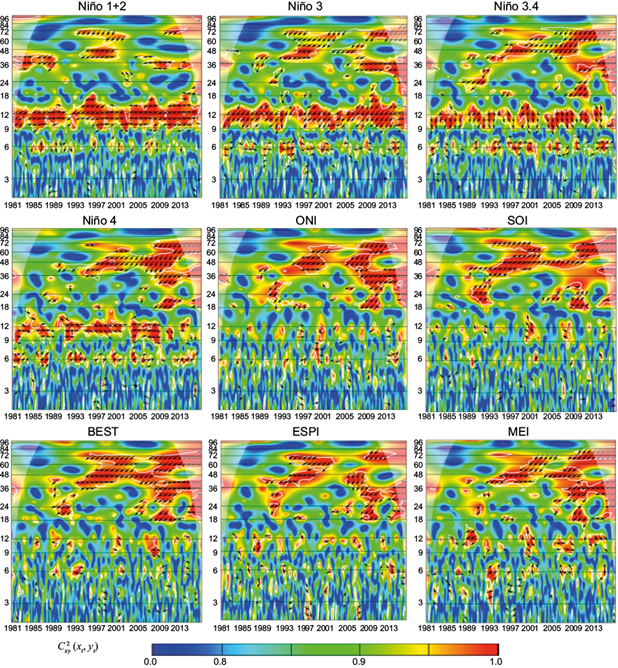
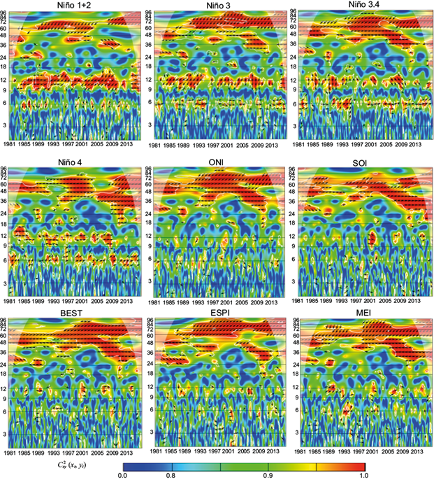
Fig. 10 Wavelet coherence C 2 x,y (x t , y t ) and phase difference Arg (T x,y (τ,s)) between ENSO indices and precipitation of Matitas station. The cone of influence is the area outside of the with a concave-down shape, and sectors of significant periodicities at 5% are enclosed by the thick white lines. Data from IDEAM. (Anti-phase: ←; In-phase: →).
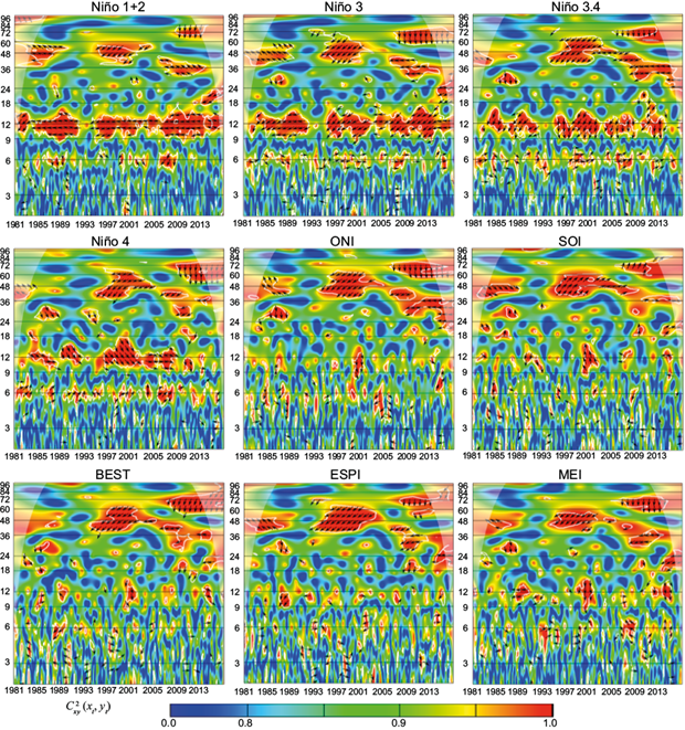
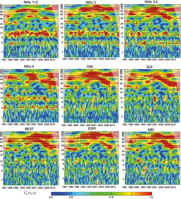
Fig. 11 Wavelet coherence C 2 x,y (x t , y t ) and phase difference Arg (T x,y (τ,s)) between ENSO indices and precipitation of Mompos station. The cone of influence is the area outside of the with a concave-down shape, and sectors of significant periodicities at 5% are enclosed by the thick white lines. Data from IDEAM. (Anti-phase: ←; In-phase: →).
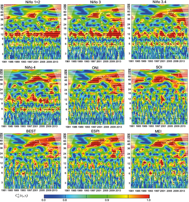
Fig. 12 Wavelet coherence C 2 x,y (x t , y t ) and phase difference Arg (T x,y (τ,s)) between ENSO indices and precipitation of Mesopotamia station. The cone of influence is the area outside of the with a concave-down shape, and sectors of significant periodicities at 5% are enclosed by the thick white lines. Data from IDEAM. (Anti-phase: ←; In-phase: →).
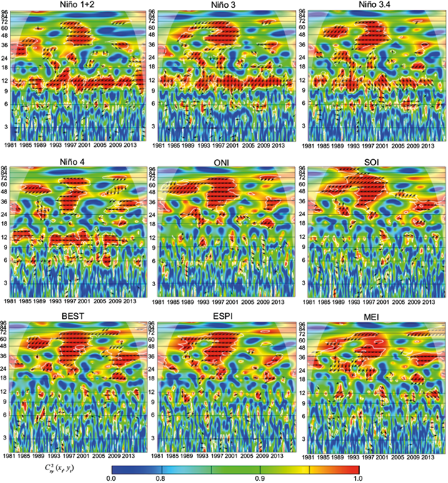
Fig. 13 Wavelet coherence C 2 x,y (x t , y t ) and phase difference Arg (T x,y (τ,s)) between ENSO indices and precipitation of Cimitarra station. The cone of influence is the area outside of the with a concave-down shape, and sectors of significant periodicities at 5% are enclosed by the thick white lines. Data from IDEAM. (Anti-phase: ←; In-phase: →).
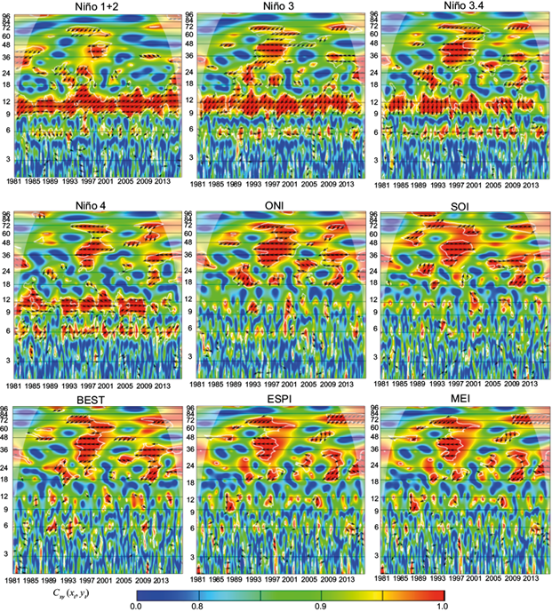
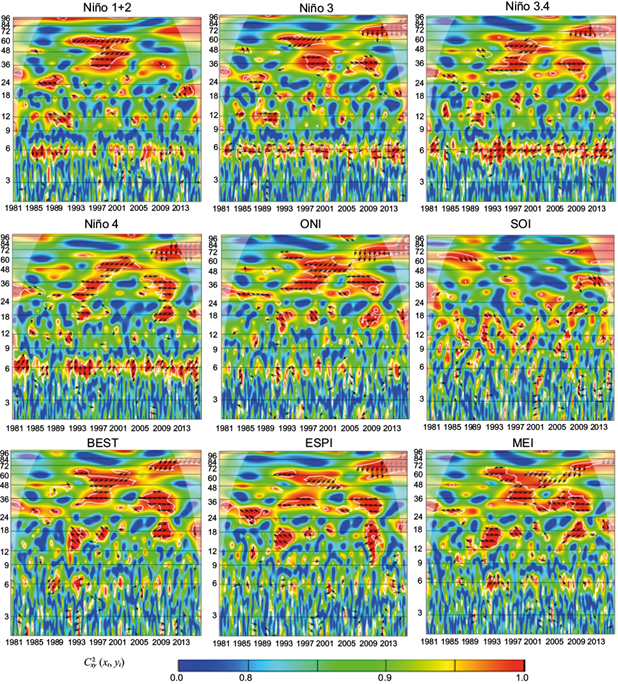
Fig. 14 Wavelet coherence C 2 x,y (x t , y t ) and phase difference Arg (T x,y (τ,s)) between ENSO indices and precipitation of Iser Pamplona station. The cone of influence is the area outside of the with a concave-down shape, and sectors of significant periodicities at 5% are enclosed by the thick white lines. Data from IDEAM. (Anti-phase: ←; In-phase: →).
The WC procedures were computed between the monthly precipitation anomalies from IDEAM data and ONI, MEI, SOI, BEST, ESPI, and MEI data. Results are shown in in the last five panels in Figures 9 to 14.
Step 4 is repeated but with the CHIRPS precipitation data. Results are shown in the first four panels in Figures A1, A2, A3, A4, A5 and A6.
Step 5 is repeated but with the CHIRPS precipitation data. Results are shown in the last five panels in Figures A1 to A6.
3. Results and Discussion
Figures 6 and 7 show the continuous wavelet spectra of the monthly precipitation data from IDEAM and CHIRPS respectively. Figure 6 displays the intraseasonal, seasonal, and interannual components in the signals. The spectra of the stations show a different precipitation variability at each location. Esperanza and Matitas have clear annual, and semi-annual cycles, the power on these scales stands out more than the others. Mompos and Mesopotamia also have an annual cycle, but the semi-annual cycle decreases its power. In contrast, in Cimitarra and Iser Pamplona, the semi-annual cycle’s power exceeds the annual.
On the inter-annual scale, the period is different for a different station. For example, La Esperanza has a significant area between 2000 and 2015 above the 32-months, and another between 1985 and 1995 above 64 months. Matitas has an area of maximum power around 1985. Mompos have homogeneous areas at interannual scales; no particular periodicity stands out. In contrast, Mesopotamia has three distinguishable areas, one between 32 and 64 months before 2000, and two between 16 and 32 months after 2000. Finally, Cimitarra and Iser Pamplona have only one great area on scales between 16 and 32 months after 2005. From Figures 2 and 3, it is appreciated that the location of significant areas coincides with strong or very strong ENSO events. However, not all stations indicate the same degree of influence. For example, La Esperanza, Cimitrarra, and Iser Pamplona correspond more with strong La Niña events in their precipitation signals, while Matitas and Mesopotamia reveal a greater coincidence with El Niño, and Mompos, has a homogeneous response.
These results are in line with previous findings about ENSO effects across Colombia (Díaz and Villegas, 2015; Beltrán and Díaz, 2020; Navarro-Monterroza et al. (2019) Poveda et al., 2020; Salas et al., 2020). These studies all affirm that ENSO’s influence depends on the intensity and the longitudinal location of the maximum SST anomaly over the Pacific and the region of Colombia that is analyzed, even stations with similar geographic coordinates and elevation can be influenced differently. The effects are not always homogeneous (Díaz and Villegas, 2015; ENA, 2018; Beltrán and Díaz, 2020). Those findings that have been verified first through linear correlations are clearer with the wavelet spectra of Figure 3 because it is appreciated over time and at different periodicity scales how annual and semi-annual variability are similar. However, at interannual and longer scales, each station has its power distribution for each frequency component. The reason is that for each site, the effects of orography, proximity to the Caribbean, to the Amazon, local circulation systems are combined and added with ENSO to generate varied responses. Efforts to describe these effects in greater detail can be found, for example, in the recent works by Navarro-Monterroza et al. (2019) and Poveda et al. (2020)
In Figure 7, we can see periodicities of 6 and 12 months in all cases using CHIRPS data, different for results using the IDEAM data, where such periodicities are not always visible. In contrast, the zones with significant periodicity greater than 12 months have less power than that revealed with the IDEAM data.
Figure 8 shows the continuous wavelet spectra of the ENSO indices. The first four spectra are for the SST of the different regions Niño 1+2, Niño 3, Ñino 3.4, and Niño 4. The annual cycle stands out with greater power, the semi-annual cycle is more evident with Niño 3.4 and Niño 4 compared to Niño 1+2 and Niño 3. The last four spectra correspond to ONI, SOI, BEST, and MEI indices, based on anomalies as described in Table I, therefore, they do not present an annual or semi-annual component. In higher scales, the power distribution reveals that each index has a greater sensitivity to warm or cold events, compared with Figure 2, the indices with greater power for El Niño events are ONI, ESPI, and MEI, and for La Niña is BEST. Studies carried out to compare the indices using linear techniques revealed that each index tends to represent better warm or cold events. For example, it has been found that El Niño 1 + 2 is more sensitive to contributing positive anomalies and Niño 4 to negative ones (Hanley et al., 2003; Yu et al., 2015; Nikreftar and Sam-Khaniani, 2018; Ballari et al., 2020). Therefore, to analyze ENSO’s impact at a specific site, it is highly recommended to identify which indices show a better relationship with the local interannual climate variability (Nikreftar and Sam-Khaniani, 2018; Ballari et al., 2020).
Figures 9 to 14 show the wavelet coherence and phase difference obtained with data from IDEAM at the six stations described in Table II. Figures A1 to A6, included in Appendix A, show the results computed with CHIRPS data. Note that the general coherence structure with both databases is very similar, but the phase difference is not always coincident; the description that follows is for Figures 9 to 14.
For Esperanza station, the coherence spectra show periodicities of 6-12 along the time, but it is particularly evident with the Niño 1+2, Niño 3, Niño 3.4 and Niño 4. The direction of the arrows changes for each index and periodicities; for example, around 12 months, arrows indicate anti-phase relationships with El Niño 1+2 and El Niño 3, then show a phase difference reduction for El Niño 3.4 and finally an in-phase with El Niño 4. For the remaining four indices, as expected, the annual and semiannual cycles are not evident. The significant sector located for the 24-36 month periodicities is present between 1985 and 1995; for most cases, the direction of the arrows implies that the index leads the precipitation. The next significant sector located between periodicities of 24-36 months occurs around 2008-2010 and is especially apparent with Niño 4, ONI, and SOI indices; the direction of the arrows also implies that the index leads the precipitation.
For Matitas station, the coherence spectra show the annual cycle of Niño 1+2, Niño 3, Niño 3.4 and Niño 4 indices. The direction of the arrows is the same as for Esperanza station. The second significant sector, located at periodicities of 36-60 months, and between 1995-2005, is most noticeable with ONI, SOI, BEST, and ESPI indices, and arrows indicate an anti-phase relationship where indices lead precipitation signal. The third sector, with periodicities of 36-48 months and between 2006-2010, is especially apparent with Niño 3.4 and Niño 4, and the direction of the arrows is the same as in the previous cases. Finally, the fourth sector with periodicities of 48-64 months, and between 2009-2015, is evident for all spectra, arrows indicate an anti-phase relationship, but the lag is reduced.
For Mompós station, spectra show the annual cycle of Niño 1+2, Niño 3, Niño 3.4 and Niño 4, but the directions of the arrows are different, in this case, the arrows indicate anti-phase relation with Niño 1+2, Niño 3, and the opposite with Niño 3.4 and Niño 4. The second and third sectors are located at periodicities of 36-60 months between 1993-2002, and exceeding 48 months between 1983-198. Both sectors are observed for most of the spectra, and arrows indicate predominant anti-phase relation.
For Mesopotamia station, similar to Mompos, the spectra show the annual cycle with Niño 1+2, Niño 3, Niño 3.4 and Niño 4, and arrows change directions in each case. The second and third sectors are located at periodicities of 32-72 months between 1981-2016, and 24-36 months between 2008-2012 respectively; and are present for all indices; arrows correspond to an anti-phase relationship between signals.
For Cimitarra station, the spectra do not show a clear relationship between annual components. Spectra show small significant sectors located at periodicities of 24-48 months between 2009-2012 and another of 48-72 months between 1997-2008. In general, this station presents smaller significant areas with all indices, and the arrows have directions less consistent with each other.
Finally, for Iser Pamplona station, the spectra do not show significant coherence between annual components either. The significant sectors are located at periodicities of 36-48 months between 1995-2002, at 24-48 months between 2006-2012, and 60-72 months between 2008-2015, especially with Niño 4, ONI, SOI, MEI and BEST. Arrows suggest a negative correlation but the lag changes for each index.
As stated in the Introduction, the first objective of this work is to explore nonlinear correlations of the ENSO-precipitation relationship, particularly for specific regions where the freshwater resources have been significantly reduced during El Niño events. And the second one is to identify which indices will improve the predictability of hydro-climatological variables. Regarding the first objective, the spectra visualize the non-linear character of the ENSO-precipitation relationship; that is, ENSO events with similar characteristics generate different responses in precipitation. Moreover, the influence also changes depending on the site. The differences between the spectra in Figures 9 to 14 show that this teleconnection is much more complicated than simple linear correlation, as it has also been mentioned in studies such as those of Carmona and Poveda (2012), Restrepo et al. (2019), Navarro-Monterroza et al. (2019), Das et al., (2020), Salas et al. (2020).
For example, all stations have a bimodal precipitation regime but have particular characteristics. The three most northern ones have two dry seasons, but the first one (December-February) is more marked than the second one (June-August); also, these stations have two wet seasons, but the second one (September-November) is more intense. The other three stations have both dry and wet seasons with similar rainfall levels on average. Despite their differences in altitude, mean annual rainfall, and coefficient of variation, all of them record significant impacts during ENSO events.
The nonlinear behavior of this relationship can be attributed to several factors, such as, the nexus of ENSO with other large-scale climate oscillations, the phase combinations of the oscillatory processes are multiple, and for each one, the resulting atmospheric state is quite different (Massei et al., 2012; Nalley et al., 2016; Araghi et al., 2016; Das et al., 2020). Another aspect is that two previously classified events in the same category may not be as similar as previously thought; several studies have revealed that ENSO’s influence on the climate variability of other remote regions depends on the longitudinal position of the maximum SST anomaly over the Pacific (Zhang et al., 2015 and 2019). For example, it has been documented that El Niño events with the highest development in the central Pacific generally have linear responses on the atmospheric-ocean dynamics over the Atlantic and the American continent, but in contrast, La Niña events located especially over eastern Pacific generate nonlinear responses in these regions (Li and Lau, 2012; Zhang et al., 2015 and 2019; Whan and Zwiers, 2017). Other methodologies, such as complex networks or deep learning techniques, are being explored to understand the behavior and complexity of the ENSO teleconnections around the planet (Donges et al., 2009, Feldhoff et al., 2015).
Regarding the second objective, which was to compare the wavelet coherence spectra with different indices, the results show that the significant areas are located in time-scales that correspond to ENSO periodicities, as has also been obtained by Poveda et al. (2011), Carmona and Poveda (2014), or Restrepo et al. (2019). The quantity and size of the significant areas varies for each case considered, therefore, to study the ENSO-precipitation relation with a single index can yield partial results, as has been shown in other investigations (Ballari et al., 2020).
Other areas that are at low-frequency bands are also visible in the spectra, which could correspond to ENSO with other quasi-decadal oscillatory processes. Several studies have tried to establish connections of other climate oscillations on variables such as precipitation or flow rates. However, the cause of these significant regions has not yet been established, neither in the power spectra of the wavelet transform nor in those of coherence (Nalley et al., 2019). Something similar happens to high-frequency bands, where a combination of the ENSO signal with others such as the Madden Julian Oscillation can also be found (Torres and Pabón, 2017, Beltrán and Díaz, 2020).
Table IV and Figure A10 show sectors that are especially evident and significant at the 95% confidence interval. Also, it presents for each case the number of ENSO events with categories: very strong (VS), strong (S), or moderate (M) according to ONI index classification (https://ggweather.com/enso/oni.htm). Table IV shows that during the period considered (1981-2016), nine El Niño events occurred, which according to the classification based on the ONI index, three were very strong, two strong and four moderate. On the other hand, seven La Niña events occurred in this same period, five strong and two moderate. In total, eight of nine El Niño events occurred precisely during the periods for which joint periodicities were observed between precipitation and ENSO indices. In contrast, only three of the seven La Niña events coincided with these periods of occurrence.
Table IV Periods during which observed significant joint periodicities occurred as shown in the wavelet coherence spectra of the monthly precipitation and climate index data.
| Sector | 1 | 2 | 3 | 4 | 5 | 6 | 7 |
| Periodicities (months) | 6 | 12 | 24-36 | 24-36 | 36-48 | 36-60 | 60-72 |
| Periods (years) | 1981-2016 | 1981-2016 | 1983-1992 | 2008-2012 | 1983-1992 | 1995-2005 | 2008-2012 |
| El Niño events | 3VS,2S, 4M | 3VS,2S, 4M | 1VS,2S, 1M | 1M | 1VS,2S, 1M | 1VS,2M | 1M |
| La Niña events | 5S, 2M | 5S, 2M | - | 2S,1M | - | 2S,1M | 2S,1M |
These results are coherent with the descriptions made by Navarro-Monterroza et al. (2019), Poveda et al. (2020), Salas at al. (2020), Beltrán and Díaz (2020). Those studies affirm that the influence of warm events on precipitation seems to be greater than of the cold events, and for this reason, the coherence of the two signals increases during El Niño events. Response to La Niña events seems to be more complex to identify. Similar results have also been obtained in studies carried out in other regions of the planet (Li and Lau, 2012; Zhang et al., 2015 and 2019; Whan and Zwiers, 2017). As it was mentioned before, authors suggest that when there is a decrease in SST in the Pacific, the processes of ocean-atmosphere interaction that are generated depend on the area where the maximum cooling is located; in the central Pacific, the atmospheric response takes less time than in the eastern Pacific, because SST is colder in this zone and the reaction of the atmosphere take longer. In contrast, when there SST increases in any area of the Pacific, deep convection processes that are released in the atmosphere become evident much faster in both the central or eastern Pacific. This difference in the mechanisms of ocean-atmosphere interaction could be the key to understanding why in most of the studies, the influence of El Niño on the variability of precipitation is more evident than of La Niña (Zhang et al., 2015 and 2019; Whan and Zwiers, 2017, Navarro-Monterroza et al. (2019).
Sectors 1 and 2, that correspond to coherence in the annual and semiannual cycles are present in four of the six stations, especially with the indices Niño 1+2, Niño 3, Niño 3.4 and Niño 4, and are almost continuous over time. Sectors 3 and 5 seem to be just a single band. For the Mompos and Mesopotamia spectra, these areas are more significant than for the Cimitarra or Iser Pamplona spectra. During the periods corresponding to the sectors 3 and 5, there were four El Niño events: 1982-1983 (VS), 1987-1988(S), 1991-1992(S), and 1986-1987(M). Sectors 4 and 7 are present in the Cimitarra and Iser Pamplona spectra with all the indices, but in the case of Mompos and Mesopotamia stations, they are less distinguishable. During the periods for sectors 4 and 7, there were three events La Niña: 2007-2008(S), 2010-2011(S), and 2011-2012(M), and just one El Niño: 2009-2010(M). Finally, sector 6 is present in all spectra. There were three El Niño: 1997-1998(VS), 1994-1995(M), and 2002-2003(M), and three La Niña: 1998-1999(S), 1999-2000(S) and 1995-1996(M).
The spectra obtained with precipitation data from IDEAM and CHIRPS show that Esperanza and Matitas are the stations with the largest number of sectors with significant coherence with ENSO. In those analyzing CHIRPS data, the area and definition are greater, for example, the sectors 5, 6 and 7 appear to be a single wide band located at periodicities greater than 48 months. Mesopotamia and Cimitarra also have significant sectors, although with less area and more discontinuities. Mompos and Iser Pamplona are the ones that are less consistent with the ENSO indices.
Note that the directions of the arrows are slightly different depending on the index. For sectors 1 and 2, the phase difference varies in particular for the first four indices. Figure 15 shows how most of the arrows obtained in these sectors indicate a negative correlation between precipitation and Niño 1+2, Niño 3, and Niño 3.4 with a predominant phase shift between -π/2 and π; in contrast, correlation is positive with Niño 4 and the lag interval is -π/2 to 0. These changes in direction are interesting to understand because it reveals not just that local climate is related to the sea surface temperature but also the changes in the lag depending on each region in the equatorial Pacific Ocean. Related issues are explored in Navarro-Monterroza et al. (2019). For sectors 3 to 7, directions are more similar among all the spectra.
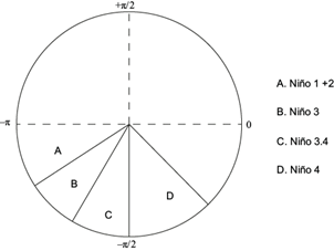
Fig. 15 Predominant phase shifts for periodicities of 12 months. Negative correlation with indices: Niño 1+2, Niño 3, Niño 3.4, and Positive with indices Niño 4.
The direction of the arrows of spectra in Figures 9-14 and A1-A6 are coincident except in the range from 36 to 48. Figures 9-14 indicate anti-phase signals with a lag of π /4, while those of A1-A6 show anti-phase signals without lag. That is, between 3 and 6 months of difference in lags calculated with each database. One possibility to understand this result is the reduced presence of anomalies in the CHIRPS series associated with ENSO events, which can modify the calculation of the phase difference. This reduction in recorded anomalies is due to the effect of combining in-situ observations and satellite data. However, the CHIRPS database also includes in-situ information, but there are large regions where there is no information, and the imputation of the data in these areas becomes difficult.
This difference occurs in all stations, and the only index that shows a minor discrepancy is ESPI, which is precisely also calculated from satellite precipitation data (Table I). To date only Urrea et al. (2016) have validated the CHIRPS data for Colombia, so it is the first time that is evident that the phase difference calculated between ENSO and precipitation changes depending on the database used, particularly on the scale of 36 to 48 months. Other validation studies have found that CHIRPS presents difficulties in estimating data from places located above 1000 m.a.s.l (Rivera et al., 2018); however, the six stations had lower and higher elevations and the discrepancy remained. This aspect should surely be the object of a more extensive and detailed investigation in future work.
Although all the indices could be used to feed statistical forecast models according to the results obtained, each station has one or more with which significant sectors of maximum coherence with greater area and definition of the phase difference were obtained. In Esperanza, ONI, Matitas with BEST, Mesopotamia with ONI or BEST and for Mompos, Cimitarra, and Iser Pamplona an option would be Niño 3 ONI and BEST.
The unique aspect of the present work is applying a non-linear method to explore relationships between ENSO and precipitation anomalies using two databases that are of different origin, although not completely independent. The results allow us to affirm that the exploration of non-linear connections obtained with each database is consistent. In other words, it was possible to identify synchronicity of the precipitation series of both databases with ENSO indices. This represents an opportunity to evaluate regional climate anomalies on the national territory where there is not enough in-situ information.
The most innovative contribution was to identify that for periods from 36 to 48 months, there is a distinction between the phase differences recorded with the IDEAM data and those of CHIRPS, and that this does not exist when both the precipitation and indices data contains satellite information.
Considering that there are two more extensive databases, more wavelet coherence between the ENSO indices was computed, the graphs in Figure 16 count the percent of spectra with each of the seven sectors chosen concerning the total of stations, which were 300 with IDEAM data and 1250 with CHIRPS. Figure 16 helps to visualize that the structure of wavelet coherence at the national level is similar both with the Pacific SST series and with the other indices. The main differences lie in the phase difference between the signals, which varies according to the database. Future work consists of expanding the scope to the whole country, finding an explanation for the change in the phase difference with the satellite data, and performing a wavelet analysis filtering bands of specific periods related to ENSO and for particular seasons where the influence is maximum like December-February.
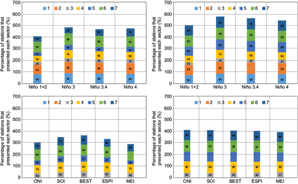
Fig. 16 Percentage of stations that presented the seven sectors described in Table IV with significant periodicities at 5%. Left: Data from IDEAM, Right: CHIR.
4. Conclusions
The purpose of exploring non-linear aspects of the ENSO-precipitation relationship is achieved by wavelet coherence analysis. The reasons for the non-linear character of the influence of ENSO on the climate variability of different regions have been attributed to the superposition of the ENSO signal with other large-scale oscillations and the influence of the longitudinal position of ENSO on the type of ocean-atmospheric response. The spectra obtained show the ENSO-precipitation relationship and also that wavelet coherence and phase difference change from one index to another. Results also indicate that the ENSO-precipitation relationship is diferent for each estation.
In the spectra, sectors of lower and higher frequency than those associated with ENSO are also visible and can be related to other climate oscillations not yet explored. The results show that ENSO years are reflected in the precipitation as periods of rainfall deficit or excess, also that precipitation is organized in bands and that most of their variance is explained by the 2-8-year scales. The most significant sectors are those that cover El Niño events, while sectors are smaller during La Niña, implying that impacts on precipitation tend to persist longer during warm events. The location of the seven most recurring sectors coincides with times in which the greatest rainfall anomalies in Colombia have occurred, and which have been associated respectively with El Niño event of 1997-1998, La Niña of 2010-2011, El Niño of 1982-1983, and La Niña of 1988-1989. Spectra also diplay, for the annual cycle, changes in the phase difference between SST of different regions and precipitation. The most influenced site have been La Esperanza y Matitas, followed by Mesopotamia y Mompos, while Cimitarra and Iser Pamplona have less influence. The indices with which significant coherence was maxima were Niño 3, ONI and BEST. The comparation of results using two different datasets (IDEAM and CHIRPS) showed that the coherence structure was similar but found discrepancies of in the phase difference in particular between 36 and 48 months.