


 nueva página del texto (beta)
 Inglés (pdf)
 Artículo en XML
 Referencias del artículo
 Enviar artículo por email
 Citado por SciELO
  Similares en
SciELO
Similares en
SciELO 
 Permalink
1. Introduction
The atmosphere is a complex system with interactions at different temporal and spatial scales. Studies of these interactions are necessary since their influen ces on atmospheric circulation can explain abnormal events in various regions of the globe. Teleconnection patterns, in which local anomalies influence remote areas, are a great example of this mechanism.
The Quasi-Biennial Oscillation (QBO) is a tele connection pattern that occurs in the tropical stratosphere. It is characterized by the almost periodic alternation between easterly and westerly winds, called, respectively, the easterly and westerly QBO phases (Ebdon, 1960, 1975; Reed et al., 1961). The cycle of zonal wind oscillation varies from 22 to 34 months, with an average of around 28 months (Baldwin et al., 2001). Naujokat (1986) described the main characteristics of QBO: the signal propagates downward to the lower stratosphere with time; the wind speed decreases at lower levels; the amplitude and the period of this oscillation change reason- ably from cycle to cycle; the transition between easterly and westerly phases occurs between 30 and 50 hPa; the easterly QBO phase is, in general, more intense than the westerly one, and during the westerly phase, the winds propagate downwards faster, favoring the prevalence of this phase for a longer time in lower levels of the stratosphere. Although QBO is not literally a biennial oscillation, there is a preferential season for phase reversal. Considering the 50 hPa level, the onset of both the easterly and westerly phases occurs mainly in the late austral autumn (Dunkerton, 1990).
In the extratropics, the Annular Modes stand out as the leading mode of climate variability. This teleconnection pattern describes north-south “seesaws” of atmospheric mass between the high latitudes and parts of the midlatitudes in both hemispheres. In the Northern Hemisphere (NH), it is known as Arctic Oscillation (AO) or Northern Annular Mode (NAM), while it the Southern Hemisphere (SH), is named Antarctic Oscillation (AAO) or Southern Annular Mode (SAM). This pattern’s structure is very similar for both hemispheres, occurring all months in the troposphere. The SAM reaches its “active phase” - maximum intensity in the stratosphere - at the end of austral spring, whereas for the NAM this stage occurs during the boreal winter. The positive (negative) Annular Mode phase is characterized by negative (positive) anomalies of geopotential height over polar regions and positive (negative) anomalies at mid-latitudes (Gong and Wang, 1999; Thompson and Wallace, 2000). This mode of variability is an active research area (Schenzinger and Osprey, 2015; Fogt and Marshall, 2020). The influence of lower frequency modes on SAM is a path to better knowledge about this pattern. Kodera and Koide (1997) and Baldwin and Dunkerton (1999) indicate that the typical NAM signal first appears in the stratosphere and then propagates downwards, suggesting that the NAM phase could be influenced by stratospheric circulation.
Although it is a tropical phenomenon, the QBO influence on the extratropical regions has been investigated by several authors, mainly in HN (e.g., Holton and Tan, 1980, 1982; Baldwin and Tung, 1994; Coughlin and Tung, 2001; Naoe and Shibata, 2010; Kuroda and Yamazaki, 2010; Roy and Haigh, 2011; Anstey and Shepherd, 2014; Li et al., 2020). Holton and Tan (1980) showed that the geopotential height at high latitudes is significantly lower during the westerly QBO phase. They suggested that the QBO may act either to focus planetary wave activity toward high latitudes or to allow its passage into the Tropics, through modulation of the latitudinal extent of the winter westerlies. The easterly QBO increases extratropical confinement of wave activity, weakening the vortex. The opposite situation during the westerly QBO, strengthens it (known as the Holton-Tan effect).
Studies relating QBO and Annular Modes have been carried out before, but they are generally focused on HN. Holton and Tan (1980), when examining 50 hPa geopotential composites in the NH, generated from the QBO phases, found a similar pattern to NAM. Coughlin and Tung (2001) showed a statistically significant relationship between the QBO signal and each level of the NAM, from 10 mb to 1000 mb, in which they all peak with the same frequency as the QBO. Other studies reveal that the positive (negative) NAM phase is associated with the westerly (easterly) QBO phase (e.g., Ruzmaikin et al., 2005; Scaife et al., 2014; Anstey and Shepherd, 2014). Kuroda and Yamazaki (2010) investigated the influence of the 11-year solar cycle and the QBO on the SAM in late winter/spring. They found that the SAM signal is strongly affected by both the solar cycle and the QBO. The SAM signal was restricted to the troposphere and disappeared very quickly in years with low solar activity.
Several studies have indicated the separate influence of QBO (e.g., Gray, 1984; Mukherjee et al., 1985; Jury et al., 1994; Peings et al., 2013; Gray et al., 2018) and SAM (e.g., Gillett et al., 2006; Silvestri and Vera, 2003, 2009; Carvalho et al., 2005; Reboita et al., 2009; Vasconcellos and Cavalcanti, 2010; Blázquez and Solman, 2017; Rosso et al., 2018; Vasconcellos et al., 2019) around the globe. As discussed above, the QBO-NAM relationship has been addressed by previous studies, indicating an association between them. However, few studies show the association between QBO and SAM (e.g., Roy and Haigh, 2011; Anstey and Shepherd, 2014). It is, therefore, necessary to verify whether this relationship also occurs in the SH and investigate its variability, to better understand the variability of SAM.
In this study, we specifically focused on evaluating the possible relationship between QBO and SAM patterns through statistical analysis. As part of this investigation, the following questions were addressed:
Is there a relationship between QBO and SAM?
Does this relationship occur on all months?
Are there lags between them?
These questions were investigated by comparing QBO and SAM indices, the latter on different levels of the troposphere and stratosphere. The Continuous Wavelet Transform (CWT) and Cross Wavelet Transform (XWT) techniques were applied to identify significant common power and phase difference between the QBO and SAM. Contingency tables and composite analyses were also used to complement the study.
This paper is outlined as follows. Section 2 introduces the datasets and describes the methodology used to investigate the association between QBO and SAM. Section 3 presents and discusses the main findings. Summary and conclusions are presented in Section 4.
2. Dataset and Methods
Monthly datasets of ERA-Interim reanalysis from the European Centre for Medium Range Weather Forecasts (ECMWF) were used for the following variables: geopotential height at 700, 200, and 30 hPa, and zonal wind at 30 hPa. The daily ERA-Interim dataset was also used for air temperature and meridional wind at 30 hPa. ERA-Interim features a global spatial coverage, with a horizontal resolution of 0.5º x 0.5º latitude/longitude and 60 vertical levels from the surface to 0.1 hPa. Details on the data assimilation system of ERA-Interim can be found in Dee et al. (2011). The 1981-2010 period was evaluated. Monthly anomalies were constructed for each month by subtracting the corresponding 1981-2010 climatological monthly mean.
The QBO index was calculated based on Naujokat (1986): zonal mean (0º -360º) of 30 hPa zonal wind at 0º latitude. The index has negative values in the easterly QBO phase and positive values in the westerly QBO phase. The SAM indices were calculated for three different levels (troposphere and stratosphere): 700, 200, and 30 hPa. The index (for each level) was obtained from the principal component time series of geopotential height monthly anomaly polewards of 30ºS, using Empirical Orthogonal Function (EOF) (Vasconcellos et al., 2019). Positive (negative) values of the SAM index are associated with negative (positive) geopotential height anomalies over Antarctica and positive (negative) geopotential height anomalies at midlatitudes.
The wavelet transform can be used to analyze time series that contain nonstationary power at many different frequencies (Daubechies, 1990). Torrence and Compo (1998) indicate that the wavelet transform allows the identification of the dominant modes of variability with a more significant contribution to the signal observed in a given period. In time or space, the CWT has movable windows, which expand or compress to capture low and high-frequency signals, respectively. Thus, it becomes a useful tool to capture the contribution of each frequency to the time series, even if that contribution varies throughout the series (Labat, 2005). CWT was applied to the SAM index time series (for each level), to find the different scales that contribute to the SAM’s large variability. The CWT figures display the time series on the X-axis and the frequency on the Y-axis. The cold colors represent less contribution to the series, and the warm colors are the frequencies that most contribute to the signal variability (high power). The CWT has edge artifacts because the wavelet is not entirely localized in time. It is, therefore, useful to introduce a Cone of Influence (COI) in which edge effects cannot be ignored. Here, the region outside of COI is in blurred shade. The Monte Carlo test wats applied to find a 90% confidence level of the signal.
The XWT displays the regions in which the two time series vary together and reveals information about the relationship between their phases through phase vectors. It means that even if the relationship between the two signals does not occur simultaneously, the XWT can identify it. The XWT allows to identify the similarity between two signals, quantifying the degree of the relationship between them over time (Labat, 2005). The XWT was calculated using QBO and SAM indices (for each level). The figures obtained from the XWT are similar to those obtained with CWT. Peak power locations correspond to regions where the time series are related. The XWT figures also have arrows, the phase angles that indicate the lag between the two time series. To analyze the phase angles, it is necessary to know which time series was processed first, and in this case, QBO was the first. The phase relationship is shown as arrows, with in-phase pointing right, anti-phase point ing left, the QBO leading SAM by 90º (270º) pointing straight down (up). The toolbox based on the methodology described in Grinsted et al. (2004) was used to calculate both CWT and XWT (available in http://grinsted.github.io/wavelet-coherence/).
Further analysis was performed comparing QBO and SAM with no lag. The SAM is a result of the sum of influences at diverse time scale (Schenzinger and Osprey, 2015; Fogt and Marshall, 2020). As QBO is a low-frequency pattern, to compare these two series, the SAM index for each level was filtered to exclude high-frequency variability, using a moving average filter. The moving average is a simple linear filter that converts a series X t , into another series Y t , by the linear operation (Equation 1):
where q and s represent the limits of the sum, and for this study q = s. X t represents the series to be filtered, Y t the resulting series, and a r are the weights used in the moving average. In this study a r is given by the expansion of the term (1/2+1/2)2q. In this way, the weight of the terms closest to the center is higher, giving them greater importance. For the 24-month (2-year) filter, the corresponding q is 12. However, for larger q values, the terms farther from the center get smaller and become negligible for the calculation. Therefore, when filtering the series, q = 4 was used, a sufficiently large value. This methodology was based on Chatfield (2004). Because of this q value, applying this filter to the first and last four months of the analyzed period is impossible. Thus, the filtered SAM index for the 1981 to 2010 period started in May 1981 and ended in August 2010.
Monthly contingency tables between the QBO and SAM (filtered) indices were created (without lag). The 2x2 tables were used. The upper-left square corresponds to the negative SAM phase events during the easterly QBO phase; the upper-right square corresponds to the negative SAM phase cases during the westerly QBO; the bottom-left square corresponds to the positive SAM phase along easterly QBO; and the bottom-right square corresponds to occurrences of a positive SAM phase along westerly QBO. These tables were created for each SAM index (700, 200, and 30 hPa). Because of the moving average filter, the contingency tables of January-April and September-December had 29 observations. The other months had 30 observations.
The correlation between the SAM index and zonal mean, both filtered using the moving average filter described above, was calculated to complement the results. The latitude versus pressure profile of this correlation was built. A t-student test (Wilks, 2006) was applied to composites at a 90% confidence level.
Geopotential height anomaly at 30 hPa and zonal wind were also filtered using the moving average filter described above. These were used to generate composite analyses for each QBO phase (without lag). The zonal wind was taken to create a latitude versus pressure profile (zonal mean). The geopotential height anomaly at 30 hPa was shown on a polar stereographic map. Also, we calculated the meri dional heat flux (v'T') at 30 hPa from the daily dataset and built composites for easterly and westerly QBO. Trenberth (1991) showed that the meridional heat flux (v'T') is proportional to the Eliassen-Palm vertical component. Edmon et al. (1980) suggested the Eliassen-Palm flux components denote the direction and magnitude of the planetary wave propagation, so 30 hPa could be used as a measure of the activity of the waves entering the stratosphere. As for the other composites, the flux was also filtered.
Since November is the active period of SAM (Thompson and Wallace, 2000), we choose this month to analyze the correlation and composites described above. The periods used for these composites were identified with the CWT of the SAM index at 30 hPa (1987-1990 and 2000-2004, see Section 3 - Results). A t-student test (Wilks, 2006) was applied to composites and correlations at a 90% confidence level.
3. Results
As mentioned, the CWT technique was applied to SAM indices at 700, 200, and 30 hPa, and results are shown in Figure 1. Warm colors in Fig. 1 have higher power, corresponding to where most of the energy in the series is concentrated, and the black line represents the 95% significance level. The analysis of the 700 hPa SAM index (Fig. 1a) shows peak power in the 1-6 months band in several tyears of the time series, ceasing around 2007. It also presents high power regions in the 1-2 year band, for the periods: 1985-1990, 2000-2003 and 2007; a peak is also seen in the 4-6 year band, between 1993 and 2001. The CWT for the 500 hPa SAM index was quite similar to Figure 1a (not shown). In the upper troposphere (200hPa - Fig. 1b), the SAM index exhibited simi lar power peaks as in the lower troposphere, but generally for shorter periods. Peaks were observed in the 1-2 year band around 1989, 2000-2004 (this peak extended longer than 2-year band) and 2007. Significantly higher power in the 4-6 year band extended from approximately 1995 to 2001. The CWT obtained for the stratospheric SAM index (30 hPa) presented differences compared to tropospheric ones, as shown in Figure 1c. First, the significant peaks in power in the band up to 3 months were less frequent. Significant high power was observed in the bands around 6 months-1 year, 1-2 years (this peak also extended longer than 2 years), while the 4-6 years band had no significant power. Significant high power in the 1-2 year band was observed in periods 1987-1990 and 2000-2004. Fogt and Marshal (2019) discuss the variability in the SAM and show that this variability stems from changes in the extratropical atmospheric circulation from the surface up through the stratosphere. Phenomena with several timescales can cause these changes, from synoptic (e.g., positive feedback between transient eddies and polar jet) to low-frequency modes (e.g., QBO and El Niño-Southern Oscillation), consistent with our CWT results.
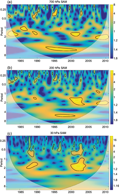
Fig. 1 Power spectrum of the continuous wavelet transform (CWT) of SAM index at: (a) 700 hPa, (b) 200 hPa, and (c) 30 hPa. The thick black contour designates the 5% significance level and the cone of influence (COI) where edge effects might distort the picture is shown as a blurred shade.
Figure 1 revealed that the SAM index had several bands of high power, indicating many sources of variability. Schenzinger and Osprey (2015) and Fogt and Marshall (2020) also suggested sources with various timescales influencing the SAM. In addition, the SAM indices showed variability near the 2-year band for both the troposphere and stratosphere, suggesting that the QBO pattern could influence SAM variability in this band.
To verify this possibility, the XWT was applied between QBO and SAM indices (for 700, 200, and 30 hPa SAM indices). Figure 2a, corresponding to the XWT between QBO index and SAM index at 700 hPa, shows intense power peaks in the 2-year band around 1984-1985, 1988-1995, and from 1999 to the end of the time series. This result indicates an association between these two patterns in this band (approximately two years). When analyzing the phase vectors, lag phases can be seen between the QBO and SAM index time series. In the 2-year band (red rectangle) for the 1984-1985 period, the vectors are inclined approximately 90º (6 months lag) and 0º (in-phase), respectively. In the period 1988-1991, the phase vectors changed from 180º (anti-phase) to 90º (6 months lag). The 1992-1995 period had vectors in-phase (around 0º). In 1999, the patterns had 6 months lag (~90º) and, in 2000 became again in-phase (around 0º). The 2001-2004 period presented a higher phase difference, approximately 270º (18 months lag). From after 2004 until the end of the time series, the patterns were in phase (around 0º). The corresponding analysis with SAM index at 500 hPa (not shown) and 200 hPa (Fig. 2b) were similar to 700 hPa.
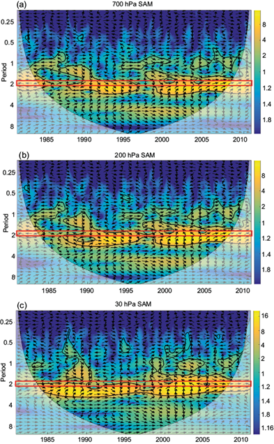
Fig. 2 Cross-wavelet transform (XWT) of the QBO and SAM index time series. The thick black contour designates the 5% significance level. The relative phase relationship is shown as arrows, with in-phase pointing right, anti-phase pointing left, the QBO leading SAM by 90º (270º) pointing straight down (up). The red rectangle displays the 2-year band.
Some differences were observed in the stratospheric XWT (30 hPa - Fig. 2c) compared to the tropospheric ones (Fig. 2a-b). The high power observed in the stratosphere (around 2-year band) was more intense than in the troposphere. As in the troposphere, 1984 had about 6 months lag in the stratosphere. While in the stratosphere the period 1985-1987 was in phase, only 1985 was significant in the troposphere. In the 1988-1989 period, the vectors inclined approximately 270° (18 months lag) and 180° (anti-phase), respectively. Although the 2-year band had no significance in 1990-1992, there was a significant area right below 2-year (still within the QBO period) in which the arrows were in phase. The 1993-1996 and 1999 periods presented a 6-month lag (around 90º). In the 2000-2005 period, the vectors had a counterclockwise rotation, starting at 0º (in-phase), passing through the 270º (18-month lag) in 2001-20002, and 180º (anti-phase) in 2003-2004, finishing at 90º (6-month lag) in 2005. From 2006 onwards, the patterns were in phase (around 0º) as in the troposphere.
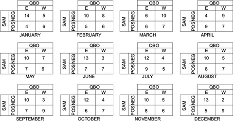
Figure 2 shows that there are different lags between QBO and SAM, including no lag; thus, we complement these results focusing on no lag. Monthly contingency tables counting the occurrences of simultaneous cases (no lag) of QBO and SAM phases (filtered) are shown in Figures 3, 4 and 5 (700, 200, and 30 hPa SAM index, respectively). It is noteworthy that the frequency of the SAM phases related to QBO phases varied slightly through the atmosphere. Perhaps this behavior occurred because the Annular Mode signal first appears in the stratosphere and propagates downwards with time (Kodera and Koide, 1997; Baldwin and Dunkerton, 1999), but that in the same month the propagation may not have yet reached the lowest levels. Additionally, Kuroda and Yamasaki (2010) indicate that the SAM signal stays restricted to the troposphere in years with low solar activity, which could also explain troposphere-stratosphere differences. It is necessary to observe the behavior of the SAM relative to the phases of QBO to analyze the contingency tables since the QBO is the longer-lasting phenomenon. Inspection of the columns in each table identified which SAM phase was more frequent in each QBO phase, to establish a relationship among them. When a SAM phase occurred more frequently during the easterly QBO and, during the westerly phase, the opposite SAM phase was more frequent (“oblique behavior” in the contingency tables), a relationship between the phenomena is suggested. Table I summarizes the results from the contingency tables (Figs. 3-5). The most frequent pattern presented the negative SAM phase related to the easterly QBO phase and the positive SAM phase associated with the westerly QBO phase. Months not included in the table did not present the “oblique behavior”.
Table I Summary of results presented in the monthly contingency tables (Fig. 3-5). Months not included in the table are those that do not present the “oblique behavior”.
| Easterly QBO/negative SAM Westerly QBO/positive SAM | Easterly QBO/positive SAM Westerly QBO/negative SAM | |
| 700 hPa SAM index | January, May, June, July, September, October, November, December | - |
| 200 hPa SAM index | January, June, July, August, September, October, November, December | April |
| 30 hPa SAM index | January, May, July, August, September, October, November, December | March, April |
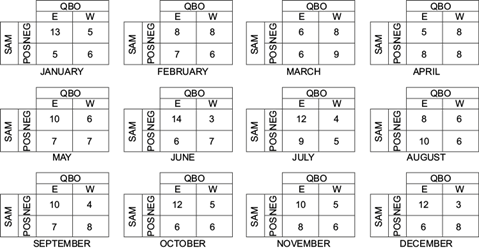
Fig. 3 Monthly contingency tables between the QBO and SAM indices. SAM index (filtered) calculated for 700 hPa. The upper-left square corresponds to the events of the negative SAM phase during the easterly QBO phase (E); the upper-right square corresponds to the cases of negative SAM phase during the westerly QBO (W); the bottom-left square corresponds to events of positive SAM phase along easterly QBO (E); and the bottom-right square corresponds to occurrences of a positive SAM phase along westerly QBO (W).

November is the active SAM period (Thompson and Wallace, 2000), so we choose this month to ana lyze the latitude versus pressure profile of correlation between the SAM index and zonal wind (both filtered) (Figure 6). The most significant correlations were found in the extratropics. This result was expected since the SAM is the leading mode of the extratropical region (Thompson and Wallace, 2000). The correlation map highlighted the relationship between SAM phase and the polar stratospheric vortex and polar night jet, showing a significant strengthening (weakening) of the stratospheric jet during positive (negative) SAM phase, as discussed in previous work (e.g., Thompson and Wallace, 2000; Fogt and Marshall, 2019). There was also a significant positive co- rrelation in the tropical stratosphere, i.e., positive (negative) SAM phase related to westerly (easterly) wind, although, at levels higher than 30hPa, this tropical region is dominated by the QBO. This result agreed with the contingency tables, indicating a relationship between positive (negative) SAM phase and westerly (easterly) QBO phase.
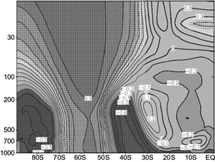
Fig. 6 Latitude versus pressure profile of correlation between the SAM index at 700 hPa and zonal wind (both filtered) for November. Areas with 90% significance are dotted (t-student test).
We also analyzed composites of geopotential height anomaly at 30 hPa for each QBO phase (Fig. 7). The period of these composites was identified from the CWT of the 30 hPa SAM index as no lag (1987-1990 and 2000-2004 - Fig. 2c). Table II shows the years used for each composite. Although there were few areas with statistical significance, the geopotential height anomaly composites displayed positive (negative) anomalies at polar (middle) latitudes for easterly QBO phase, indicating negative SAM phase. The westerly QBO composite presented the opposite pattern, suggesting a positive SAM phase. These composites confirmed the results from the contingency tables.
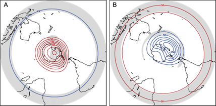
Fig. 7 Composite of geopotential height anomaly (m - filtered) for 30 hPa: (a) easterly QBO, and (b) westerly QBO. Contour interval of 25 m. Areas with 90% significance are shown in shaded (t-student test).
Table II Classification of easterly and westerly QBO years (November) used for composite analysis (Figure 6). The period analyzed is 1987-1990 and 2000-2004.
| Easterly QBO | Westerly QBO |
| 1988, 1989, 2000, 2001, 2002, 2003 | 1987, 1990, 2004 |
Although the scope of this work was not to investigate the mechanisms of the QBO-SAM relationship, a possible cause of this link is wave propagation to the stratosphere, which affects the QBO and the polar stratospheric vortex (e.g., Baldwin and Tung, 1994; Thompson and Wallace, 2000; Fogt and Marshall, 2019; Li et al., 2020). The maximum of this wave propagation from the troposphere to the stratosphere in the SH occurs in late spring (Charney and Drazin, 1961; Randel and Newman, 1998). To corroborate this hypothesis, we analyzed the composites of meridional heat flux at 30 hPa for November (Fig. 8). The composites were built for the period described in Table II. Edmon et al. (1980) discussed the role Eliassen-Palm flux components to identify the direction and magnitude of the planetary wave propa- gation. The meridional heat flux is proportional to the Eliassen-Palm vertical component (Trenberth, 1991), and it can be used to measure the activity of the waves entering the stratosphere. Maximum nega- tive values occurred at 60ºS, and there was almost no difference between QBO phases at this latitude (Fig. 8). However, at higher latitudes where the polar stratospheric vortex was located, the easterly QBO displayed stronger values, which suggested there was more wave propagation to the stratosphere in this phase, compared to westerly QBO. Li et al. (2020) also indicated stronger (weaker) upward wave propagation to the stratosphere with easterly (westerly) QBO and linked this to the polar stratospheric vortex. The wave develops in the troposphere and propagates vertically into the stratosphere along the jet core axis. The wave decelerates the stratospheric polar jet by depositing easterly momentum into the westerly stratospheric jet (Charney and Drazin, 1961; Edmon et al., 1980; Randel and Newman, 1998; Kuroda and Yamazaki, 2010). Figure 9 confirmed the stratospheric jet weakening in the easterly QBO composite. A weak (strong) stratospheric jet is associa- ted with a negative (positive) SAM phase (Thomson and Wallace, 2000; Fogt and Marshall 2020). The results presented above confirmed the relationship between QBO and SAM and indicated upward wave propagation to the stratosphere at high latitudes as a possible mechanism.
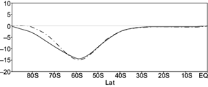
Fig. 8 Composite of zonal mean meridional heat flux (K ms-1) for 30 hPa. Solid line: easterly QBO, and dot dashed line: westerly QBO.

4. Summary and conclusions
The SAM pattern influences climate over the SH (e.g., Gillett et al., 2006; Silvestri and Vera, 2003, 2009; Vasconcellos et al., 2019). However, the varia- bility of this mode is an active area of research. The influence of lower frequency modes on SAM is a path to better knowledge about its variability. While prior works have studied the relationship between QBO and NAM, few studies showed an association between QBO and SAM. This study confirmed that this relationship also occurs in the SH and investigated the variability associated with this relation.
CWT applied to SAM indices in the troposphere and stratosphere, showed power peaks for different bands, including around 2 years. In the stratosphere (30 hPa), the significantly higher power around the 2-year band was seen for the periods 1987-1990 and 2000-2004. This result indicated SAM index had variability at various scales, including two-years, possibly because of the QBO influence. The XWTs analysis between the QBO and SAM indices revealed significant common high power around the 2-year band for all the results obtained. However, this band showed lag variations between the QBO and SAM series over the analyzed period, including no lag., suggesting that the influence of the QBO on the SAM could happen simultaneously and several months later.
Focusing on the QBO influence on the SAM with no lag, we built monthly contingency tables between the QBO index and the SAM indices at different levels (30, 200, and 700 hPa - filtered, without lags). These results showed that, for most of the months, during the QBO easterly phase, there was a higher occurrence of the negative SAM phase. Alternatively, during the QBO westerly phase, there was a higher occurrence of the positive SAM phase. This relationship between QBO and SAM is consistent with previous results (e.g., Roy and Haigh, 2011; Anstey and Shepherd, 2014). Nevertheless, this study showed that this relationship is not valid for all months. Composite analyses for each QBO phase (period described at 30 hPa SAM`s CWT) were performed for the SAM active period (November), confirming the results from the contingency tables. More (less) upward wave propagation into the stratosphere at high latitudes for easterly (westerly) QBO phase, weakening (strengthens) the stratospheric polar vortex, leading to negative SAM phase. These results agree with results by Fogt and Marshall (2020) and Li et al. (2020).
This study confirmed that there is a relationship between the QBO and the SAM. It also showed various lags between these two patterns, suggesting that this relation has a complex interaction. Nevertheless, analyses without lag indicated that the ne- gative (positive) SAM phase was more frequent for easterly (westerly) QBO in most (but not all) months, including the SAM active period (November). It lies beyond the scope of this study to determine the physical mechanisms associated with the influence of QBO on SAM. However, some additional analy-sis indicated that the upward wave propagation to the stratosphere for each QBO phase modifies the stratospheric jet and, consequently, the SAM phase. This study provides insight on SAM variability and its predictability. Further research is ongoing and will be presented in future publications.

