


 nueva página del texto (beta)
 Inglés (pdf)
 Artículo en XML
 Referencias del artículo
 Enviar artículo por email
 Citado por SciELO
  Similares en
SciELO
Similares en
SciELO 
 Permalink
1. Introduction
The Amazon basin is definitely one of the major convective activity areas across tropical regions worldwide. The corresponding convective rainfall keeps a close relationship with the local and regional behavior of dynamic and thermodynamic variables, which are also influenced by global atmospheric phenomena, such that those factors should be considered when evaluating rainy and dry seasons (Wang et al., 2017; Spracklen et al., 2018; Cavalcante et al., 2019; Molina et al., 2019).
Complementarily, the Amazon ecosystem is also directly connected to ancient and nowadays precipitation cycles. Paleoclimatological analyses reveal that different plant species are highly dependent on a certain amount of paleo-precipitation meaning that a decrease of this variable makes the region more prone to savanization (Wang et al., 2017).
Due to the influence of climate change on rainfall events and also to the evolution of land use and land cover, monitoring rain variability is essential to estimate and mitigate the effects of those changes over the Amazon ecosystem. Deforestation and climate change can both contribute to severe damages on the forest ecosystem, notably in the Amazon forest biome, resulting in a loss of biodiversity, reduction of the corresponding carbon retention capacity, and soil weakness, eventually impelling the Amazon to a gradual process of savanization (Pielke, 2005; Zemp et al., 2017; Le Page, 2017; Schielein and Börner, 2018).
Another important remark is that the Amazon region presents a pluviometric station network with at least two significant problems or limitations, namely the irregular density and the great number of gaps in the historical data series. The area of the Amazon region in the Brazilian territory, which englobes about 5 500 000 km², has barely 613 rain gauges with a collection area of the equipment that, added up, cover an area of measurement (not taking into account its area of influence) of approximately 24.5 m2, whichis only 4.46 × 10⁻¹⁰% of the measurable territory (ANA, 2018).
In this sense, rainfall estimates from space sensors present an opportunity to complement the standard observational network and allow the development of real-time applications. However, the benefits of those estimates can only be used if they are properly validated and if their accuracy is adequately described (Mantas et al., 2014).
Under this framework, the use of different techniques for the pluviometric description comes up as a possible solution, such as the information basis provided by orbital remote sensing, since it allows to retrieve observations from almost all the parts of the Earth in relatively small time intervals, contributing to a better understanding of rainfall in regions where there are no satisfactory in situ observational networks or even in the case there is no rainfall observation at all (Liu and Peter, 2013).
Different studies have been developed to address precipitation behavior in the Amazon region and South America based on comparisons between rainfall historical series derived from rain gauges and satellite datasets, as conducted by Nóbrega (2008), Pereira et al. (2010, 2015) and Paiva et al. (2012), among others. However, those studies did not explore in-depth the representativeness and identification of the various frequency cycles and spatio-temporal trends that could be found in the rainfall datasets. On the other side, rainfall products have also been explored as input to hydrological models, as investigated, for instance, in the study by Correa et al. (2017). In this case, it should be pointed out that such type of analysis usually fails to rigorously validate the quality of the input dataset. In general, the option is to calibrate and validate the model-generated stream flows against observed recorded stream flows using mathematical objective functions, not necessarily considering the adequate representation of the spatio-temporal field of rainfall.
It should also be emphasized that adequate rainfall monitoring is quite important not only for rainy time periods and flooding but also for droughts with a variety of applications at the watershed management level such as agricultural and irrigation projects and hydropower operation and planning,
Trejo et al. (2016) explored the performance of satellite rainfall product CHIRPS (Climate Hazards Group InfraRed Precipitation with Station data) in contrast to ground observed rainfall over Venezuela in the 1981-2007 period with respect to their accuracy in drought and flood periods. The assessment was made by usual performance measures such as Pearson correlation coefficient, mean error, relative mean absolute error, Nash-Sutcliffe efficiency coefficient and percent bias, jointly with standard categorical metrics such as probability of detection and false alarm ratio. Overall evaluation was that the satellite product overestimated lower monthly rainfall values whereas it underestimated higher values (> 100 mm × month-1), with moderately high coherence between satellite rainfall estimates and rain gauge observations. Moreover, the authors indicate that the satellite product misclassified rainfall events and they do not recommend using it for drought monitoring in Venezuela due to the high uncertainty in identifying presence or non-presence of precipitation, especially when the rainy season is taken into account. Instead, they suggest the use of drought indices such as the standardized precipitation index (SPI), which is based on cumulative rainfall.
By examining some of the constrains of the previously cited studies, the wavelet technique emerges as an alternative to explore more thoroughly rainfall datasets, some of them previously examined in published evaluations under different methodological frameworks. It should be emphasized that this work provides new insights concerning signal analysis, which could be grouped basically into two domains: time scale (frequency or period) and location of disruptive variations along the time series. Therefore, wavelet analysis allows to establish standards of comparison to determine specific variations that might have occurred in a given time scale and location in the historical time series (Kang and Lin, 2007). Besides that, the application of wavelet transform englobes the analysis of time series that might be non-stationarity at different frequencies (Torrence and Compo, 1998), being suitable for comparing low-frequency variability along historical time series.
In order to summarize, this study intends to fulfill the existing knowledge gap in terms of providing a full analysis of the rainfall performance in the Madeira river basin, encompassing rainfall and non-rainfall courses based on four remotely perceived products, specifically: (i) Climate Hazards Group InfraRed Precipitation (CHIRP), (ii) Climate Hazards Group InfraRed Precipitation with Station data (CHIRPS), (iii) 3B42, and (iv) 3B42RT from Tropical Rainfall Measuring Mission (TRMM), together with rain-gauge data available in the locality. Furthermore, the transformed wavelet analysis was applied to the rainfall datasets to consider a complementary verification of the representativeness of the cycles and frequencies associated with precipitation in this sub-basin and its coherence with the rainfall remote sensing estimates in the region. The paper is organized as follows: section 2 describes the study area and the characteristics of the rainfall datasets, jointly with the procedures for defining the methodological approach to address rainfall patterns at the Madeira river watershed; results for the proposed procedures are presented in section 3, and finally section 4 presents a brief summary and concluding remarks.
2. Materials and methods
2.1 Study area
The Madeira river basin (Fig. 1) is located southwest of the Amazon River (right bank) and it is one of its main affluents. This sub-basin presents international limits, thus being a transboundary basin that extends through Bolivia (51%), Brazil (42%) and Peru (7%), with a total drainage area of 1 324 727 km2. Actually, the referred basin represents the largest Amazon sub-basin (23%).
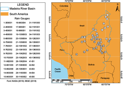
Fig. 1 Location of the study area: Madeira river basin and corresponding available rain gauges (pluviometric stations) used in the analysis (2001-2015).
According to the Köppen classification, the basin presents three climate zones: Af: tropical humid to super humid; Am: tropical rainforest, with monsoon rainfall and a dry season of short duration, and Aw: tropical warm, with a dry winter season (Peel et al., 2007). Two typical seasons are identified in the region: the rainy season from October to April and the dry season from May to September.
2.2 Rainfall database
The period of analysis, which comprises the years 2001 to 2015, was chosen due to: (i) it encompasses more stations with data available without gaps within the area of the Madeira river basin, and (ii) there are also simultaneous remotely sensed rainfall products available, namely 3B42 and 3B42RT from TRMM (1999 to 2015), and CHIRP and CHIRPS, both from 1981 to the present.
2.3 Surface data
The information was collected in the Brazilian and Bolivian territories. In Brazil, the information of volumes precipitated is collected at the daily scale and obtained by means of rain gauges installed and operated by the Brazilian National Water Agency (ANA) in partnership with the Brazilian Geological Survey (SGB), more specifically, the Brazilian Company of Mineral Resources Research (CPRM), in the form of historical time series available in the Brazilian HidroWeb system (ANA, 2018). The information from the Bolivian territory was collected in monthly accumulations through a request to the National Service of Meteorology and Hydrology of Bolivia (SENAMHI).
However, because of the low density of the rain-gauge network within the Amazon region and the numerous periods with data failures, the analysis was performed based on a quantitative set of 40 historical time series of Brazilian rain gauges, labeled according to the registration number defined by ANA (Fig. 1) and five stations in Bolivia, which are named B1, B2, B3, B4 and B5 (Fig. 1).
The selected time series had less than 30% of monthly missing data. The missing monthly accumulated data were filled by the ordinary kriging interpolation method, which is based on the principle of the best linear unbiased estimation (Journel and Huijbregts, 1978). The spherical model, which is one of the positive-definite functions commonly used in geostatistics, is adopted in this study.
The kriging procedure uses a continuous function that explains the behavior of a variable in the different directions of a defined geographical area, and allows to associate the variability of the estimation based on the distance that exists between a pair of points, by the use of a semivariogram, assuming second-order stationarity. It should be noted that the semivariogram is the mathematical description of the relationship between the behavior of the variance for groupings of pairs of rainfall observations ranked accordingly to the distance separating such pairs of observations (h). The expression of the empirical omnidirectional expression for the semivariogram, which is the basis for modeling a continuous function for posterior implementation of the interpolation kriging procedure, is given by
where: γ̂ (h) is the estimated semivariogram, N(h) the number of pairs of measured values at a certain distance h, and z (.) the observation value located at a certain point x.
2.4 Remote sensing data
This work evaluates four satellite rainfall products: (i) Climate Hazards Group InfraRed Precipitation (CHIRP), (ii) Climate Hazards Group InfraRed Precipitation with Station data (CHIRPS), and the products (iii) 3B42 and (iv) 3B42RT from the Tropical Rainfall Measuring Mission (TRMM). The remote sensing data CHIRP and CHIRPS are provided by the Climate Hazards Group (CHG, http://chg.geog.ucsb.edu/data/chirps/). These products have more than 30 years of data (beginning in 1981) in spatial resolutions ranging from 0.25 to 0.05º for the quasi-global coverage of 50º S to 50º N. Both CHIRP and CHIRPS are based on a global 0.05º monthly precipitation climatology (CHPclim). The formulation of CHPclim consists of the incorporation of physiographic features (elevation, latitude and, longitude) and monthly average data acquired from satellite. CHPclim satellite data include microwave precipitation estimates from TRMM 2B31, microwave-plus-infrared precipitation from Climate Prediction Center MORPHing (CMORPH), monthly infrared brightness temperatures from geostationary source, and land surface temperature (Funk et al., 2015).
In addition to CHPclim data, CHIRP uses cold cloud duration (CCD) data, which is the time interval in which a temperature pixel is below a certain threshold, based on satellite Thermal InfraRed (TIR) images. It is assumed that rainfall and CCD are linearly correlated. The calibration of CCD data uses 5-day rainfall from the Tropical Rainfall Measuring Mission Multi-satellite Precipitation Analysis (TMPA 3B42), which has a spatial resolution of 0.25º (Funk et al., 2015). Each pentadal precipitation estimate is then converted to the fraction of the long-term mean precipitation estimate. Lastly, fractions are multiplied by the CHPclim value, generating the CHIRP product. Daily precipitation estimates are generated by redistributing the pentadal totals in proportion to the daily 0.05º grid of the Coupled Forecast System. CHIRPS differs from CHIRP because it incorporates rain-gauge stations data through the use of a modified inverse distance weighting algorithm. More information concerning CHIRP and CHIRPS can be found in Funk et al. (2015).
Two products from the TRMM satellite, the 3-h near-real-time (TMPA 3B42RT) and the research-grade (TMPA 3B42) were analyzed in this study. Both products are provided by NASA (https://mirador.gsfc.nasa.gov) at the same 0.25º × 0.25º resolution. The 3B42RT considers only satellite data for precipitation estimates and is available since March 1, 2000 while 3B42 data is based on 3B42RT with ground data and is available since January 1, 1998 (Liu, 2015).
The TMPA dataset considers two main data sources for rainfall estimates. The first is precipitation-related microwave data extracted from numerous orbital sensors onboard the Low Earth Orbit (LEO) satellites (Huffman and Bolvin, 2018). The second is infrared (IR) data from the international constellation of geosynchronous (geo) satellites (Huffman and Bolvin, 2018).
The general methodology to retrieve TMPA 3B42RT data can be divided into three steps (Huffman et al., 2010; Huffman and Bolvin, 2018): (1) the microwave data are converted to precipitation estimates at 3-h time scale using different Goddard Profiling Algorithms, depending on the sensor (see Huffman and Bolvin, 2018), and combined; (2) the IR data are calibrated through histogram matching of the microwave precipitation estimates (Duan et al., 2016), and (3) microwave- and IR-based estimates are merged (the IR-based estimates are used just to fill out missing data in the microwave estimates).
The TMPA 3B42 data requires the integration of the above-mentioned data with the rain-gauge data. In this process, all the microwave-IR merged precipitation estimates are summed into monthly totals creating a multi-satellite (MS) product. The MS data is combined with the Global Precipitation Climatology Centre (GPCC) monthly rain-gauge analysis (Rudolf et al., 1994) products using the inverse-error-variance weighting, which generates the monthly TRMM product (3B43) (Huffman et al., 2010). Lastly, the 3-h precipitation estimates are adjusted for each month, making their sums equal to the TRMM 3B43 (Huffman et al., 2010). Thus, the adjusted precipitation is the final 3B42 product. More details concerning the TMPA algorithms can be found in Huffman et al. (2010) and Huffman and Bolvin (2018).
To compare with observed daily rain-gauge data, satellite estimates were accumulated during daily periods according to the reading reference of rain gauges, i.e., of the amount collected along 24 h initiating at 7:00 LT on the day of record. Subsequently, data were accumulated at a monthly time scale.
2.5 Analysis of rainfall patterns and data grouping
The analysis to characterize pluviometric patterns among the available stations in order to identify rain-gauge clusters accordingly to common features regarding the rainfall regime and their geographic relation, other than investigating and identifying any sort of existing spatial pattern, had also the purpose of systematizing the comparison of observed data with satellite estimates, including the examination of their behavior along the time in the frequency space with respect to localized intermittent periodicities by means of the wavelet transform technique.
The hierarchical cluster method, which is the most used technique in this type of evaluation (Andrade et al., 2016), was used in this process. The method consists of grouping the pluviometric stations by a process that was sequenced at several levels until a dendrogram is established, which is a simplified representation of the dissimilarity matrix.
The Ward method was chosen as a technique for group formation. In this technique, the distance between two clusters is the sum of the squared deviations of the points to the centroids. The objective of the Ward link is to minimize the sum of squares within the pool. The distance is calculated with the distance matrix of Eq. (2) based on the expression
where d mj is distance between groups m and j; m is the merged cluster consisting of clusters k and l, with m = (k, i); d kj is the distance between clusters k and j; d lj is the distance between groups l and j; d kl is the distance between clusters k and l; N j is the number of variables in grouping j; N k is the number of variables in grouping k; N l is the number of variables in cluster l, and N m is the number of variables in the cluster m.
Finally, the square of the Pearson correlation coefficient (r²) (the coefficient of determination) defined at the magnitude level of 70%, was the criterion used for the formation of groups and dendrogram cutting.
2.6 Comparison between rain gauges and remote sensing database
The virtual station (pixel centroid) was used as remote sensing information for evaluations with the rain-gauge data. The comparison was made between the rain gauges and the nearest virtual station. The area represented by a virtual station depends on the satellite pixel size, which is 0.25º for 3B42RT and 3B42, and 0.05º for CHIRPS and CHIRP. As the Amazonian rain-gauge network is sparse, none of the pixels had more than one rain gauge for comparison. The analysis scale was monthly.
2.7 Deterministic assessment of satellite estimates
A dispersion matrix of the analyzed data series was built, where each of the data sources was graphically placed with another series to evaluate the relationship between them.
Three analysis groups were made in order to verify the efficiency of the remote sensing data, containing: (i) the total quantitative historical series, (ii) months representing the dry period in the region (April to September), and (iii) months constituting the rainy season (October to March). Inside each analysis group, the following metrics were studied: standard error (E) (Eq. 3); coefficient of determination (r²) (Eq. 4), and Willmott’s concordance index (Willmott et al., 1985) (Eq. 5), as well as the derived performance index, which is the product between the Pearson correlation coefficient (r) and the Willmott concordance index (d). The classification accordingly to the intervals of the performance index is presented in Table I. Below are the expressions for E, r² and d, given, respectively, by
where x E is the estimated event average, x M are the measured events average, and N is the total number of validation stations.
Table I Classification of the performance index.
| Performance index | Classification |
| > 0.85 | Great |
| 0.76-0.85 | very good |
| 0.61-0.75 | Good |
| 0.61-0.65 | Median |
| 0.51-0.60 | Affordable |
| 0.41-0.50 | Bad |
| ≤ 0.40 | Awful |
Source: Willmott et al., 1985.
Stations B1, B2, 965001 and 1063001 served as controls to test the level of accuracy achieved by what we call “raw datasets” CHIRP and 3B42RT, in order to describe the historical rain-gauge series, since they are not contaminated due to insertion of corrections and adjustments with in situ observational rainfall data taken into account.
2.8 Wavelet transform
As previously mentioned, the wavelet transform is a technique used to reveal the periodic characteristics of non-stationary variance at different time scales (Torrence and Compo, 1998). It also allows the identification of the main periodicities in a time series and the progression in time of each frequency (Liang et al., 2011). In this context, this technique was used to compare the characteristics of the historical rain-gauge time series and the corresponding pixels in terms of rainfall estimated by remote sensing products (3B42, 3B42RT, CHIRP and CHIRPS) in the time-frequency domain. The technique was applied to the averages of the series of stations within each defined group during the grouping analysis. There are many families of waving functions. In particular, the Morlet function (Eq. 6) is recommended for hydrological studies, mainly pluviometric series, because it has a similar pattern to the sign of this variable, revealing peaks and ranges in wavy signals similar to rainfall data (Brito, 2013). It can be expressed by
where s is the scale of the wavelets and H (ω) is the Heaviside step function. H (ω) = 1 if ω > 0, H (ω) = 0 if ω < 0; the dimensionless frequency (ω0) was considered equal to 6 to satisfy the admissibility condition, providing a good balance between time and frequency location (Grinsted et al., 2004).
The methodology combines the techniques of coherence by wavelets (WTC), which indicates the covariance between two-time time series as a function of time-frequency, and the crossed wavelet (XWT), which shows a power spectrum that indicates the regions of interference between two-time series (Brito, 2014).
3. Results
3.1 Grouping analysis
The grouping analysis of the monthly rain-gauge data performed between 2001 and 2015 resulted in the dendrogram shown in Figure 2. It can be observed that the threshold defined for a correlation considered strong between stations (> 70%) determined the existence of four homogeneous groups, represented graphically by different colors.
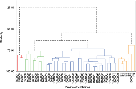
The spatial distribution of the 45 stations in the four homogeneous groups is shown in Figure 3, which also shows the hypsometric basin map on a logarithmic scale to better observe the differences in elevation. The arrange of the groups is based on the proximity of stations and on the elevation profile.

The monthly average rainfall of each group is presented as histograms in Figure 4. All groups indicate the existence of a dry season starting in April, with an increase in precipitation from November until the end of March.
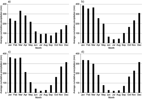
Fig. 4 Monthly mean precipitation histograms: (a) cluster 1, (b) cluster 2, (c) cluster 3, (d) cluster 4.
Clusters 2, 3 and 4 show that January to March are the rainiest months, while in group 1, March stands out from the others and the rainier quarter would be February-March-April. August presented the lowest rainfall in all groups. The study of Andrade et al. (2016), when analyzing the same basin using data from 41 rainfall stations in a historical time series between 1978 and 1998, found a similar cluster configuration, thus confirming a degree of stationarity in the pluviometric characteristics of the region.
It is worth noting that cluster 1, which presented anomalous features by its contrast through the main data from the other clusters, is located at the lowest part of the basin near its extort (i.e., next to the confluence of the Madeira river with the Amazon river). This region was pointed out by Souza (2019) as a region that had a great recurrence of La Niña events in the last 30 years, which caused extreme rainfall episodes with high return periods (low frequency events).
3.2 Efficiency of remote sensing sources
The comparison between precipitation accumulations observed in the pluviometric stations and estimated by CHIRP, CHIRPS, 3B42, and 3B42RT from 2001 to 2015 are presented in Figures 5-7. Analyzing the values of the regression coefficient for the total set of monthly accumulation historical time series (Fig. 5), it is verified that the CHIRPS data were mostly above 0.7 and slightly below for the wet period. In the dry period, products performed better with higher magnitudes of r², having the products CHIRP and 3B42 a performance evaluated with a regression coefficient of the order of 0.6. The historical time series of the product data of the 3B42RT achieved a lower level of performance since the regression coefficient was around 0.5.
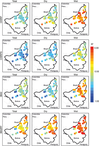
Fig. 5 Efficiency analysis: coefficient of determination (r2) for the annual total rainfall values and also for the dry (April-October) and wet (November-March) periods.
It should also be noted that the regression method approach is limited to estimate the efficiency of the TRMM data in the Amazon region for time series encompassing a limited number of years. In the case of a cyclical event, in which both time series show increases and reductions independently of the magnitudes, such variation can hide data inaccuracies.
The average standard error analysis also followed the trend of the regression coefficient (Fig. 6). It can be observed that the magnitude of these errors is inversely proportional to the amount of rainfall, a fact that was also confirmed by the agreement index (Fig. 7), where the former was higher in the dry regions for the CHIRPS and CHIRP data, while the latter indicated that the performance of TRMM products in representing rainfall for all rain gauge stations tested in the rainy season was highly inadequate.
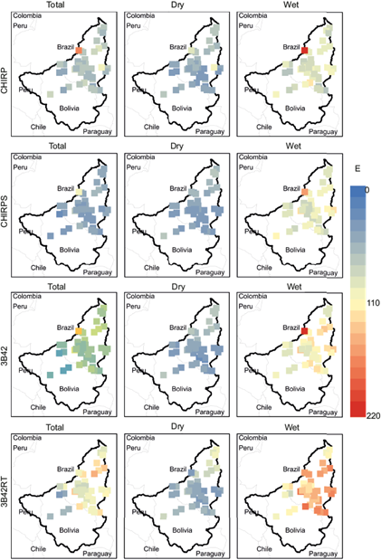
Fig. 6 Efficiency analysis: average standard error (E) for the annual total values and also for the dry (April-October) and wet (November-March) periods.
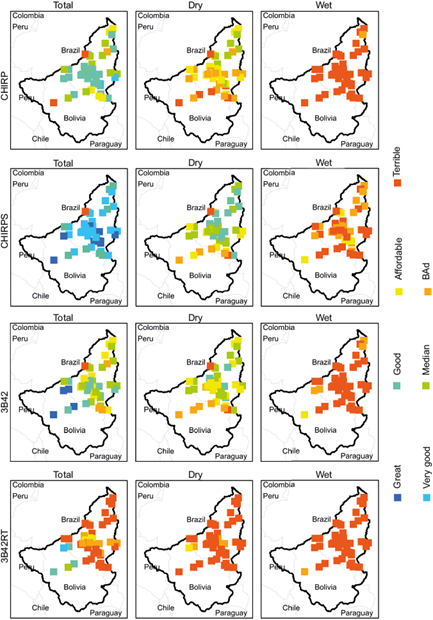
Fig. 7 Efficiency analysis: Willmott’s concordance index for the annual total values and also for the dry (April-October) and wet (November-March) periods.
The study of Paca (2008), for instance, found a similar behavior for the data of the product 3B42 in the Guamá river basin in the state of Pará (PA), Brazil, also located in the Amazon basin. In general, the differences in the performance of the products result mainly from the variation in their spatial resolution, once the pixel representation smoothes out the frequency of the most intense events (Ensor and Robeson, 2008), making the estimate more complex at coarse resolutions. For example, estimates 3B42 and 3B42RT, which are averaged over a larger area (0.25º × 0.25 º), do not represent the spatial variation of rainfall caused by differences in relief or by convection, which is provided by rain-gauge observations.
In the comparison between data estimated by remote sensing and data observed in the stations, there are two interesting facts: (1) the low correspondence of the remote sensing data with rainfall information in the rainy season, and (2) the slightly better correspondence in the dry season. The possibility of underestimating precipitation as a consequence of the pixel resolution is more evident in the rainy season. This fact explains the lower correspondence with the specific data for that period.
The information mentioned above confirms the concern of the study of Ali et al. (2003), which emphasizes that the intermittency of rainfall in the Amazon region induces a great spatial variability, which by itself causes uncertainty for point measurement to be extrapolated to represent a real average.
In this context, Sodré et al. (2012) highlighted that the possible cause of these discrepancies is a seasonal variation of large-scale phenomena and local convective processes, such as the displacement of lines of instability, which needs more in-depth studies to prove this hypothesis.
In a similar study using rain gauges and TRMM data conducted for the transition area of the Amazonian forest between 1988 and 2013, Serrão et al. (2016) showed higher r² values in rainy periods than in dry months. Therefore, there is no overall truth about the efficiency of TRMM data since it varies according to the region evaluated.
Concerning this greater effectiveness of TRMM data to describe dry periods within the Amazon region, Paca (2008) reported the highest degree of correlation observed for a region close to the studied basin in 2005, in which there was a typical rainfall pattern in the northern region when an extreme drought event occurred.
Sodré et al. (2012)) highlighted that the reliability of TRMM data should be questioned, since it presents a discrepancy of more than 100 mm in monthly values during rainy periods with respect to the amount measured in rain gauges.
Also, the type of clouds formed over the location should be taken into account in the analysis segmented by seasons. In the Amazon region, rainfall during the rainy season can originate from both shallow and deep clouds. Few clouds are observed during the dry season, and those that are formed are associated with the burning of biomass, which releases aerosols leading to large vertical non-precipitating clouds (Fish et al., 1998; Andrade et al., 2009). Thus, the greater assertiveness of products in periods of low precipitation might be linked to the accuracy of sensors and their corresponding wavelengths, whose responses are dependent on the sensitivity when interacting with water content within clouds and detecting temperature at the top of the clouds.
Algorithms to estimate satellite rainfall are based on the thermal infrared (TIR) band, inferring the cloud-top temperature, or on the passive microwave (PMW) band, which penetrates the cloud to explore internal properties through the interaction of raindrops with the radiation energy field. There are advantages and disadvantages to be considered in using either type of sensor.
TIR-based rainfall estimates present higher uncertainties in identifying the presence of some types of mixed-phase clouds or warm clouds. Therefore, cirrus clouds are frequently confused with convective clouds due to similar brightness. On the other hand, PMW-based rainfall estimates have a marked bias in the presence of warm orographic rainfall and over very cold surfaces as mountains-tops covered with snow, which is interpreted as precipitation. PMW-based algorithms may frequently outperform TIR-based techniques for instantaneous rainfall over a specific region, while TIR gives better results than PMW algorithms for longer periods.
Proceeding with a more in-depth evaluation of the results depicted in Figures 5-7, it can be said that the most efficient combination of TIR and PMW techniques in the conception of CHIRP and CHIRPS products explains their better overall performance in comparison to TRMM products. Better satellite estimates of rainfall when compared to rain-gauge observations are achieved for higher relief altitudes. Complementarily, rainy seasons are usually exposed to more complex cloud systems, leading to enlarged difficulties in producing a more accurate rainfall measurement. Dry seasons are thus expected to produce more reliable rainfall estimates with lower degree of uncertainty.
The behavior of the stations that served as control points (B1, B2, 965001 e 1063001) was similar to the results for the whole set of stations (Table II), with outstanding superiority of the CHIRPS data, followed by CHIRP information and better representativeness for periods of low rainfall.
Table II Analysis of the control points efficiency.
| Index | Database | Time series | Pluviometric station code | |||
| 965001 | 1063001 | B3 | B4 | |||
| Regression coefficient (r²) | CHIRPS | Total | 0.80 | 0.74 | 0.82 | 0.80 |
| Dry | 0.64 | 0.66 | 0.73 | 0.55 | ||
| Wet | 0.52 | 0.44 | 0.81 | 0.60 | ||
| CHIRP | Total | 0.64 | 0.63 | 0.27 | 0.64 | |
| Dry | 0.51 | 0.39 | 0.15 | 0.19 | ||
| Wet | 0.11 | 0.28 | 0.09 | 0.38 | ||
| 3B42 | Total | 0.65 | 0.54 | 0.83 | 0.88 | |
| Dry | 0.62 | 0.57 | 0.78 | 0.79 | ||
| Wet | 0.24 | 0.15 | 0.82 | 0.74 | ||
| 3B42RT | Total | 0.28 | 0.34 | 0.59 | 0.70 | |
| Dry | 0.15 | 0.26 | 0.33 | 0.47 | ||
| Wet | 0.02 | 0.11 | 0.57 | 0.44 | ||
| Average standard error (E) (mm) | CHIRPS | Total | 44.71 | 49.19 | 43.22 | 34.32 |
| Dry | 44.35 | 42.21 | 73.02 | 38.45 | ||
| Wet | 77.78 | 96.01 | 113.77 | 85.76 | ||
| CHIRP | Total | 63.51 | 64.07 | 87.07 | 68.70 | |
| Dry | 53.04 | 52.69 | 69.38 | 64.93 | ||
| Wet | 98.31 | 100.89 | 121.22 | 99.15 | ||
| 3B42 | Total | 52.11 | 57.42 | 39.92 | 29.71 | |
| Dry | 43.49 | 44.73 | 74.47 | 40.00 | ||
| Wet | 90.94 | 96.01 | 106.02 | 94.25 | ||
| 3B42RT | Total | 103.07 | 96.23 | 63.54 | 56.32 | |
| Dry | 56.76 | 55.25 | 78.34 | 55.93 | ||
| Wet | 130.83 | 132.72 | 109.00 | 111.11 | ||
| Willmott’s concordance index (c) | CHIRPS | Total | Very good | Very good | Great | Very good |
| Dry | Median | Median | Bad | Bad | ||
| Wet | Bad | Awful | Affordable | Awful | ||
| CHIRP | Total | Good | Good | Awful | Good | |
| Dry | Bad | Bad | Awful | Awful | ||
| Wet | Awful | Awful | Awful | Awful | ||
| 3B42 | Total | Good | Median | Great | Great | |
| Dry | Median | Affordable | Bad | Bad | ||
| Wet | Awful | Awful | Affordable | Awful | ||
| 3B42RT | Total | Awful | Bad | Good | Good | |
| Dry | Awful | Awful | Awful | Awful | ||
| Wet | Awful | Awful | Bad | Awful | ||
To comparatively analyze the data sources, scatter plots were constructed, as shown in Figure 8, including the dry and rainy seasons of the region.
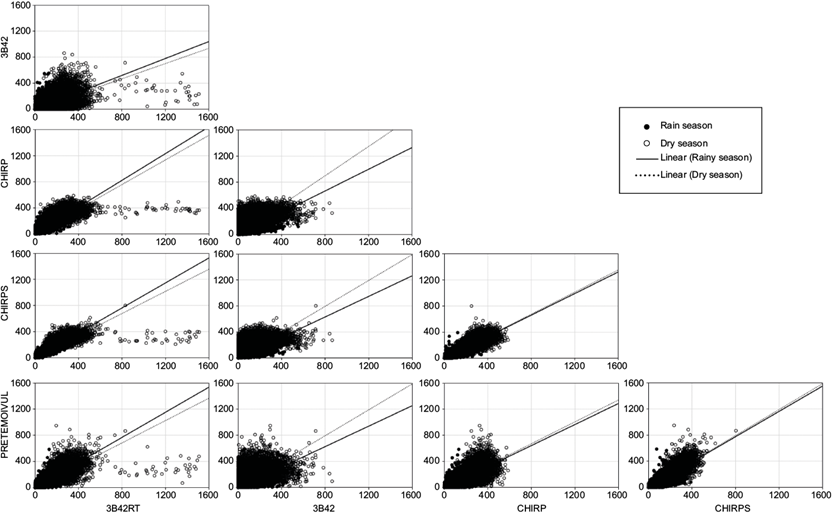
Fig. 8 Data dispersion diagrams for the dry and rainy period using in situ data (pluviometer) and the products CHIRP, CHIRPS, 3B42, and 3B42RT.
In general, the 3B42 product shows a greater dispersion than CHIRP and CHIRPS when compared with pluviometric stations. Possibly, the efficiency of the high-quality monthly rainfall climatology of CHPclim directly influences the suitability of CHIRP and CHIRPS products, since the model uses not only physiographic indicators (elevation, latitude, and longitude) but also medium-term monthly field information of five satellite products: estimates of microwave precipitation, CMORPH-based microwave and infrared precipitation estimates, average monthly temperatures of geostationary infrared brightness, and estimates of the Earth’s surface temperature (Funk et al., 2015).
The CHIRP and CHIRPS products presented the greater similarity between them, possibly because the former is a non-interpolated version of the latter, in which a network of ground stations is also considered. In addition, both products presented results close to the TRMM products, proving that the TMPA 3B42 product from TRMM has an influence in the calibration of precipitation estimates through the data of cold clouds duration (CCD) for the production of CHIRP and CHIRPS (Funk et al., 2015).
It should also be noted that the rainy seasons presented in general a more dispersed behavior, whereas, in the dry season, there is a clearer tendency of alignment of the data, as shown in the diagram, indicating better agreement between different source data and better adjustment of a tendency line.
3.3 Cycles and frequency comparisons
The results of applying the continuous wavelet transform tool to datasets are shown in Figures 9 and 10. In the generated images, colors with stronger tones denote higher power in the spectrum, while the black outlines mark the significant regions of time and periodicities for the range at a 95% confidence level. The lateral edges mark the cone of influence of edge effects for the size of the analyzed series. Both the period and the time axes are graduated in months. The time axis informs the number of months after the beginning of the time series, which is January 2001 in all cases.
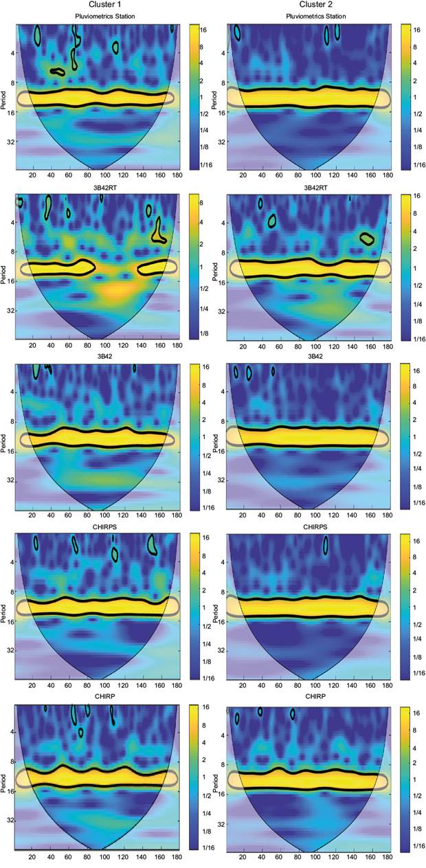
Fig. 9 Continuous wavelet transform analysis of the estimates of various sources of remote sensing data in the pixels of representative rain gauges (pluviometric stations) of clusters 1 and 2.
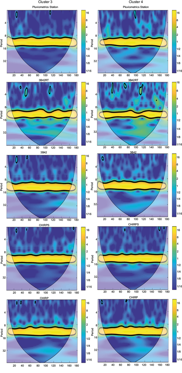
Fig. 10 Continuous wavelets transform analysis of the estimates of various sources of remote sensing data in the pixels of representative rain gauges (pluviometric stations) of clusters 3 and 4.
As expected, a periodicity around 12 months (an annual cycle) is shown as significant for the whole length of the time series for all clusters and remote sensing products estimates, except for 3B42RT. In Figure 9, cluster 1 shows an interruption localized between 90 and 130 months after January 2001 (from July 2007 to April 2011). This anomaly is specifically seen in the 3B42RT time series, showing, once again, that the corrections employed in this model caused the corresponding time series to be flawed and less representative of the Madeira river basin.
The continuous wavelet transform (CWT) analysis may reveal similar cycles and their anomalies in the individual time series but their manual localization is not precise and their similarities may be only coincidences. So, to certify the existence of the similarity, cross wavelet transform (XWT) and wavelet transform coherence (WTC) are applied to the pair of series to be compared, where the remote sensing products and the data of the rain gauges represent the clusters.
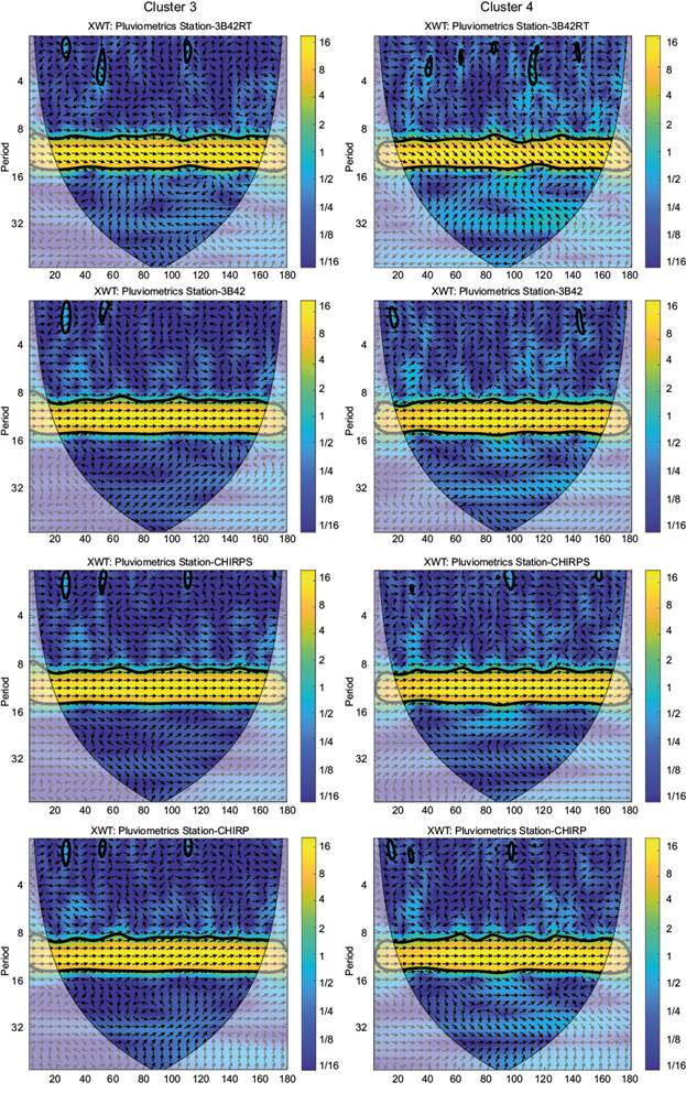
The XWT analysis (Figures 11 and 12) exposes regions with high significant common power and may reveal the phase relationship between the series, where arrows pointing to the right indicate in-phase behavior and arrows pointing left show anti-phase behavior.

The WTC analysis (Figures 13 and 14) reveals how coherent is the cross wavelet transform in time frequency space. The hotter the color, the higher the coherence between them. Also, arrows pointing to the right indicate in-phase behavior and arrows pointing left show anti-phase behavior.


In the XWT analysis, it is possible to determine the similarity between two datasets by evaluating, in the period axis, the existence of a yellowish strip at the height level 12 for the entire time interval and the presence of arrows pointing to the right, which denotes the presence of a similar annual cycle between both.
When contrasting the rain gauge and the TRMM pixel datasets in the coherence analysis (WTC), a full correlation of data close to magnitude 1 would be ideally expected. Thus, the more similar a time series is to another, the larger the zones with colors close to the yellow. Besides, the vectors should indicate that there is an agreement in phase. Thus, the rightward direction of the arrows is expected.
It is noticed that the information of CHIRPS is more representative for all clusters and periodicities (annual and interannual possible cycles) throughout the length of the time series, while the TRMM 3B42RT product showed less representativeness, mainly in interannual periods. There are large areas that denote a correlation close to 1, which indicates that an historical time series is directly proportional to another series.
In general, CHIRPS data can be considered a good option for the Amazon region, since this area has a low density of pluviometric stations. Therefore, CHIRPS can provide a qualified full coverage to assess rainfall distribution across the studied region.
Analyzing all the investigated scenarios jointly, it is noticed that the time series of pixels of all products obtained from remote sensing are sensitive to the occurrence of rainfall and climate events, with well-defined interannual variability and a great capacity to represent periods of drought in the Amazon region. Nevertheless, in rainy periods, the rainfall amount associated with areas of these pixels partially fail to accurately represent the rainfall intensity of a rainfall station, especially the so-called TRMM products (3B42 and 3B42RT).
4. Conclusions
The results indicate that satellite-estimated rainfall is a feasible alternative for accurately monitoring rainfall in the Madeira river basin, in order to complement or substitute rain gauge stations.
The analysis of rainfall data from the rain-gauge network identified four groups/clusters with similar behavior across the Madeira river basin. The rain-gauge stations in each of the clusters are geographically close and have similar elevation. Satellite rainfall estimates and rain-gauge observations were then compared using the following metrics: coefficient of determination, average standard error and Willmott’s concordance index.
Results showed that spatio-temporal rainfall distributions can be reasonably estimated by satellite; however, further research is required to improve estimates of rainfall amount. More precise satellite estimates are related to higher relief altitudes. Uncertainties are assumed to be partially due to the presence of different types of clouds in the region and partially due to limitations of the algorithms presently used in satellite platforms, which are essentially based on thermal infrared and passive microwave sensors.
The remotely sensed rainfall datasets CHIRPS and CHIRP better represent the monthly accumulated pluviometric data across the Madeira river basin, compared to the 3B42 and 3B42RT datasets. Nevertheless, the superior performance is not homogeneous, with larger uncertainty for the rainiest months. Moreover, a higher performance of satellite rainfall products was achieved for dry periods in comparison to wet periods.
Wavelets analysis was able to capture and identify more thoroughly the consistency of the rainfall time series evaluated in dry and wet periods. In particular, the technique revealed the lack of adequate representation of interannual cycles in the 3B42RT data in predefined time periods during which the analysis was conducted.
It should be emphasized that the present study provided very good results for dry periods, which is quite useful in hydrology when examining runs of drought sequences and their consequent effects in water balance at the watershed scale. It is worthwhile to further investigate this aspect, since the higher reliability of satellite products in dry periods could be more useful in terms of watershed management, including urban and rural planning associated to water supply, energy generation, and food production.
Under the perspective of looking ahead to improve rainfall estimates, which still present limitations, we should mention that new sensors and corresponding updated algorithms are currently being developed with refined spatial and temporal resolution. This will certainly represent an advance regarding accuracies and uncertainties associated with the variety of scales at which different data sets are collected. The highlighted issue is quite relevant to our case study, since we are comparing information at the pixel-spatial and rain-gauge spatial resolutions, which for comparison purposes are assumed to be a point in space.
Improved statistical and stochastic techniques such as wavelet analysis, as explored here, jointly with fractal and geostatistical approaches to integrate spatial and point information constitute viable alternatives to achieve better results in rainfall estimation based on remotely-sensed information. Statistical methods that combine spatial and local information could be better explored in future works
As a final word, we should say that satellite-derived rainfall datasets such as the ones examined in this study play nowadays an essential role in the provision of distributed quantitative data over regions with scarce or unavailable data. In this sense, society can rely on these relatively new datasets to take administrative and management decisions at city, state, and national levels integrated at the basin level, involving a diversity of areas such as hydrology, meteorology, agrometeorology, engineering construction, water supply, and sanitary treatment, among other required urban and rural planning actions.

