


 text new page (beta)
 English (pdf)
 Article in xml format
 Article references
 Send this article by e-mail
 Cited by SciELO
  Similars in
SciELO
Similars in
SciELO 
 Permalink
1. Introduction
Air quality modeling is an essential tool for most air pollution studies (Seinfeld and Pandis, 2012). In that sense, Lagrangian models provide an effective method for simulating atmospheric diffusion when chemical reactions are not relevant. Specifically, Lagrangian models can estimate the local air pollution produced by emissions from a large power plant (Souto et al., 2000). They have usually been accepted as the most adequate models for estimating the local plume dispersion from single large point sources (Souto et al., 2009). Currently, the Lagrangian modeling approach is mainly divided into two different categories: particle models and puff models (Zannetti, 2013). In this work, a comparison between two representative Lagrangian models, FLEXPART and CALPUFF, coupled to the WRF meteorological model (Skamarock et al., 2008) is performed.
FLEXPART (Stohl et al., 1998) is a widely used Lagrangian particle model that simulates the transport and dispersion of tracers by calculating the trajectories of a multitude of particles. As in some of the most recent FLEXPART model studies at different regions all over the world, Wei et al. (2011) used models coupling (WRF-FLEXPART) to describe the impact of high-pressure conditions on the air quality in northern China. Using the same model coupling, Bei et al. (2013) analyzed meteorological conditions and plume transport patterns during the Cal-Mex 2010 study in Tijuana, Mexico. Halse et al. (2013) developed a forecasting system based on FLEXPART for long-term forecast and assessment of polychlorinated biphenyls atmospheric transport in different observed air pollution episodes at remote sites in southern Norway. Also, Arnold et al. (2015) investigated the role of precipitation in the Fukushima nuclear accident (Tanaka, 2012; Yang, 2014). Besides, Djambazov and Pericleous (2015) applied the FLEXPART model to estimate how N air pollutant emissions contribute to the sea solved nitrogen in the English Channel and the south of the North Sea. Miao et al. (2015) studied the transport mechanisms of pollutants during a fog event at Bohai Bay, China, using WRF-FLEXPART models coupling to understand the effects of local atmospheric circulation and atmospheric boundary layer structure in the air pollution levels. Then, Srinivas et al. (2016) examined the sensitivity of FLEXPART to the meteorological data inputs simulated by the mesoscale model ARW in the Kalpakkam coastal environment. Newly, Cheng et al. (2017) simulated a total monthly CO2 footprint using FLEXPART.
In these studies, FLEXPART has usually been applied to long distance air pollution transport, with strong circulation patterns providing quite straight trajectories. However, FLEXPART can also be applied at a local scale in weak wind conditions. As an example, Cécé et al. (2016) modeled the dispersion of anthropogenic nitrogen oxides (NOx) emissions over the densely populated area of the Guadeloupe archipelago under weak trade winds during a typical case of severe pollution.
CALPUFF (Scire et al., 2000) is one of the most versatile and most applied Lagrangian puff models used in recent years (Hernández-Garcés et al., 2016). It is a multi-layer, multi-species non-steady-state puff dispersion model that can simulate the effects of time- and space-varying meteorological conditions on pollutant transport, transformation, and removal. CALPUFF contains algorithms for near-source effects such as building downwash, transitional plume rise, partial plume penetration, sub-grid scale terrain interactions as well as longer range effects such as pollutants removal (wet scavenging and dry deposition), chemical transformation, vertical wind shear, overwater transport and coastal interaction effects. Also, a regulatory version of the CALPUFF model is available, which tries to guarantee that model results are mainly higher than the observed air pollution levels.
As CALPUFF is a very flexible Lagrangian puff model with different solutions of atmospheric dispersion phenomena, different validation tests of the CALPUFF model have been published (O’Neill et al., 2001; Levy et al., 2003; Protonotariou et al., 2004; Cohen et al., 2005; Yau and Macdonald, 2010; Dresser and Huzier, 2011; Fishwick and Scorgie, 2011; Ghannam and El-Fadel, 2013). As some of the most recent CALPUFF studies, Rood (2014) validated CALPUFF in an industrial zone in Denver, Colorado, USA. Hernández-Garcés et al. (2015a) performed different CALPUFF assessments by simulating the local dispersion of SO2 (as a passive tracer) from a large power plant smokestack (356.5 m height, with four parallel independent pipes inside the same concrete structure), considering both different stack modeling settings (four pipers vs. one equivalent single pipe) and meteorological inputs (both meteorological models results and observations). Pivato et al. (2015) applied CALPUFF to assess the airborne concentration of an emitted pesticide. Holnicki et al. (2016) presented a case study application of the CALPUFF model at an urban scale over the Warsaw area. More recently, Fallah-Shorshani et al. (2017) simulated the pollutants transport at the top of the urban canopy using CALPUFF as part of an integrated modeling system to simulate ambient nitrogen dioxide in a dense urban neighborhood.
Apart from the mesoscale wind provided as input to any Lagrangian model, two main phenomena affect these model’s performance at the local scale: the atmospheric turbulence, as pollutant atmospheric diffusion depends on it; and the planetary boundary layer (PBL) depth, because pollutants plume rise is usually limited by this depth.
About the atmospheric turbulence effect, both FLEXPART and CALPUFF models follow the classical Lagrangian approach of increasing the element (either puff or particle) position every time step Δt by adding a vΔt distance. However, in the case of the FLEXPART particle model, v includes not only the mesoscale wind speed but also the turbulent wind fluctuations effect, in order to estimate the pollutants’ atmospheric diffusion; this FLEXPART approach is based on the parameterization scheme for statistical models proposed by Hanna (1982) and modified by Ryall and Maryon (1997). On the other hand, CALPUFF represents atmospheric diffusion using a piece-wise Gaussian distribution, as in previous adaptive puff models (Ludwig et al., 1989; Souto et al., 1998). Although CALPUFF provides several options to estimate atmospheric Gaussian diffusion parameters, the classical approach, based on the similarity theory (Monin and Obukhov, 1954), was adopted.
About PBL depth, the applied estimation with both models is based on the bulk Richardson approach of Vogelezang and Holtslag (1996) with different convective velocity scale, w*.
CALPUFF coupled to WRF meteorological model (Skamarock et al., 2008) derives this friction velocity from the vertical eddy fluxes of momentum WRF results (|w´u´|), using the Mesoscale Model Interface (MMIF) meteorological preprocessor (Brashers and Emery, 2016) that applies the Deardorff (1970) expression
where g is the gravitational acceleration, T
v
is the absolute temperature, z
i
is the average depth of the mixed layer, and
On the other hand, FLEXPART follows the convective velocity scale suggested by Vogelezang and Holtslag (1996):
where
Both w* formulations are analogous, thus similar PBL depth estimations are expected for simulations obtained with CALPUFF and FLEXPART. However, MMIF also incorporates the methodology of Gryning and Batchvarova (2003), which reduces the critical Richardson number for overwater PBL heights from 0.25 to 0.05. Therefore, in a small island domain, it is expected that overwater MMIF PBL depth will be smaller than the FLEXPART PBL depth estimation.
This is just one example of the influence of the simulation domain conditions in model assessment and intercomparison. Therefore, it is common to compare models results at different conditions. Different CALPUFF and AERMOD regulatory model comparisons were published (Dresser et al., 2011; Tartakovsky et al., 2013, 2016; Gulia et al., 2015). Also, Scire et al. (2013) added a comparison with CAMx (Tesche et al., 2001) using its plume-in-grid approach. Rood (2014) performed a comparison between the former regulatory model Industrial Source Complex 2 (US-EPA, 1992) and RATCHET (Ramsdell et al., 1994). Other researchers compared CALPUFF with different models: Yau et al. (2010) against AUSTAL2000 (VDI, 2000); Protonotariou et al. (2004) against Eulerian models UAM (Causley, 1992) and REMSAD (ICF Consulting, 2002); Chang et al. (2003) against HPAC (DTRA, 1999) and VLSTRACK (Bauer and Gibbs, 1998).
Also, some FLEXPART model comparisons were performed at long distance experiments. Probably the most comprehensive is the comparison against HYSPLIT (Draxler and Hess, 1998), CALPUFF and other two dispersion models in the European Tracer Experiment (ETEX) and the Cross-Appalachian Tracer Experiment (CAPTEX), using a tracer cloud dispersion. This last study concluded that CALPUFF performance was significantly poorer than the performance of the other three models in the ETEX experiment, while CALPUFF results were improved in CAPTEX (Anderson and Brode, 2010). At a local scale, Souto et al. (2001) compared two Lagrangian models during an SO2 air pollution episode, the Lagrangian particle model (LPM; Pielke, 1984) and the Adaptive Puff Model 2 (APM2; Souto et al., 1998), concluding that, even though vertical concentration profiles provided by LPM are more heterogeneous than estimated by APM2 (with the same meteorological input), this puff model achieved a better agreement to glc observations than LPM, as APM2 was able to reproduce observed local hotspots that were not estimated by LPM. However, previous studies at different domains indicated that Lagrangian particle models usually provide better results than other simple Gaussian puff models (Saltbones et al., 1996). Therefore, model performance depends not only on the basic modeling approach (i.e., particles vs. puffs) but also on the modeling solutions for specific phenomena (plume rise, building effects, etc.) and on the domain conditions (Hernández-Garcés et al., 2015b).
This is why in this work a singular simulation domain was selected, the Guadeloupe archipelago, including the complexity of small orographic tropical islands (width < 50 km) with strong sea influence at the Caribbean region. Particularly, from medium to weak trade winds (< 7 ms-1), its complex terrain at the Lesser Antilles may induce thermal and orographic local circulations, which strongly affect the air quality levels (Cécé et al 2014, 2016).
In this study, a comparison of the results of two Lagrangian dispersion models, FLEXPART and CALPUFF, coupled to the same meteorological fields input provided by WRF model (Skamarock et al., 2008) was done, considering NOx emissions as a passive tracer over the densely populated area of the Guadeloupe archipelago under weak trade winds, during a typical episode of severe pollution.
2. Materials and methods
2.1 Study location
The Guadeloupe archipelago is located in the middle of the Lesser Antilles arc at 16.22º N and 61.55º W (Fig. 1). This archipelago includes two main islands: Basse-Terre, a complex terrain island with a maximum elevation height of 1467 masl, and Grande-Terre, a flat terrain island with a maximum elevation height of 135 masl. The archipelago islands form a basin between the two main islands. This region is usually characterized by calm winds, but specific airflows in the atmospheric boundary layer can be observed with strong sea influence along its narrow coastline.

Fig. 1 Map of the Guadeloupe archipelago, with the main NOx emission source, a diesel power plant (PWP, red triangle), and two air quality stations near it (blue squares): AQS1 (Pointe-à-Pitre, 1878 m travel distance) and AQS2 (Baie-Mahault, 6135 m travel distance).
The main anthropogenic sources of atmospheric pollution in this region are a diesel power plant (PWP, Fig. 2) located in the center of the archipelago (Fig. 1) and vehicles on the primary road network. As this is the largest NOx emission source in the region, observed NOx glc is mainly produced by PWP emissions, so the NOx emission can be considered as a tracer of its plume. Two air quality stations near to the PWP (1878 m and 6135 m travel distances) are recording data every 15 min, which will be applied in model assessment.

2.2 Simulation period and WRF meteorological results
Cécé et al. (2016) studied a period of 24-h (1200 LT December 3-1200 LT December 4, 2007) with high NOx glc and weak winds, as the most typical meteorological conditions that produce poor air quality at the two sites available. To evaluate the performance of the two selected Lagrangian models (FLEXPART and CALPUFF) the same period was chosen for model assessment.
Meteorological input for both Lagrangian models was obtained from the WRF model (Skamarock et al., 2008) previously validated simulations (Cécé et al., 2016). Because of the complex terrain and strong sea influence around the domain, six one-way WRF nested grids (Fig. 3) were applied from 27-km horizontal resolution (D1) to 111-m horizontal resolution (D6). However, just the innermost grids WRF results (D4, D5, D6) were applied as meteorological inputs for the air quality simulations.
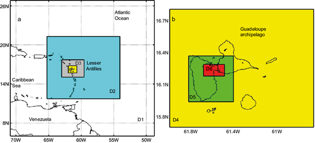
Fig. 3 WRF domain grids resolution: D1: 27 km; D2: 9 km; D3: 3 km; D4: 1 km; D5: 333 m; D6: 111 m (Cécé et al., 2016). D4, D5, D6 grids results provide the meteorological input to FLEXPART and CALPUFF air quality simulations.
Taking into account the large differences between the six grids applied, the following WRF model settings were carefully selected to get the best model performance: 70 unequally spaced half vertical eta-levels with the lowest half level at 13 meters above the ground level (magl) and the model top set at 100 hPa pressure level; Rayleigh damping on vertical velocity with a damping layer depth of 5 km; Monin-Obukhov similarity; WRF single-moment 6-class microphysics scheme; Rapid Radiative Transfer Model longwave scheme (Mlawer et al., 1997); the Dudhia shortwave scheme (Dudhia, 1989), and ensemble-mean non-local-K YSU scheme for the PBL in mesoscale domains (Hong et al., 2006).
The topography of the Guadeloupe archipelago (domains D4, D5 and D6) was interpolated from the Institut Géographique National 50-m topographic map and its land-use was interpolated from the 25-m Corine Land Cover map (EEA, 2007) pre-converted to 24 USGS land-use categories (Anderson et al., 1976; Pineda et al., 2004).
As D4 to D6 grids provide the meteorological inputs for air quality simulations, Figure 4 shows the three wind roses obtained from the corresponding grid WRF output at the PWP location. As it is observed in the three domains, changes in wind direction are covering mostly 360º, as in a weak wind condition. However, sea breeze regimes are significant, because some more frequent wind directions are observed, with differences depending on the grid resolution considered: NNE, E and ESE wind directions are the most frequent using D4 (1-km resolution) and D5 (333-m resolution) grids outputs; however, D6 (111-m resolution) grid output also shows frequent W and E wind directions. In addition, wind speed (Fig. 5) is quite different depending on the grid resolution, with frequent values up to 5 ms-1 from D4 output, which are lower from D6 output.

Fig. 4 Comparison between wind roses at the emission source location from each WRF high resolution grid output: (a) D4: 1 km; (b) D5: 333 m; (c) D6: 111 m.

Fig. 5 Wind speed time series at the emission source location from each WRF high resolution grid output: D4: 1 km (blue diamond line); D5: 333 m (red diamond line), and D6: 111 m (green triangles line).
There is more short-term variability in the D5 and D6 wind speeds, especially in the daytime. It is mainly linked with the much finer resolution and the better representation of the lower-levels daytime convection turbulence.
These differences in the WRF meteorological results depending on the grid resolution can be relevant in air quality simulations in this domain. Therefore, the same meteorological input will be set for both Lagrangian models simulations.
2.3 FLEXPART model setup
Because of the domain complexity and strong meteorological variability along with the 24-h simulation, 10-min WRF outputs are provided to the FLEXPART model, following Cécé et al. (2016). These meteorological outputs include mass-weighted time-averaged wind fields, friction velocity, heat sensible flux and PBL height. PBL turbulence is parameterized following the Hanna scheme (Hanna, 1982), which computes turbulent profiles depending on the atmospheric stability of the PBL.
According to the Pollutant Emissions French Register, PWP released 9.79 kt of NOx (equivalent NO2) in 2007. Based on this annual amount, NOx total mass emitted by PWP during 24 h is set to 26.82 t, with a constant emission rate, as no hourly profile information is available. The PWP plume is represented as Cécé et al. (2016) did using plume observational pictures (Fig. 6) by a volume of 30 × 30 × 340 m centered at 61.5515º W and 16.2280º N. The plume base corresponds with a smokestack height of 60 magl.

In the FLEXPART model, concentrations are calculated on the basis of the number of trajectories located within each grid cell and their mass fraction. The larger the number of released particles, the better represented are the particle mass fraction statistics for each grid cell. Hence, for a given resolution grid, an optimal number of trajectories to run in the model needs to be estimated. In order to determine this number corresponding to result stability, several simulation tests have been made with a number of particles released every 15 min ranging from 5000 to 60 000 particles. These tests have shown that the result stability was reached for 1-km, 333-m and 111-m grids, with the respective number of particles emitted every 15 min during the 24-h period: 20 000, 30 000 and 50 000 (Cécé et al., 2016).
NOx dispersion emitted from the PWP is simulated over domains D4, D5 and D6 (simulations: flx1km, flx0.3km, flx0.1km). As a result, NOx concentrations are computed every 15 min at the two available air quality stations, AQS1 (Pointe-à-Pitre) and AQS2 (Baie-Mahault). NOx concentrations are also computed over a three-dimensional grid, with 38 terrain-following levels (first level at 10 magl and top level at 3000 magl) and 1, 0.3 and 0.1 km of horizontal resolution, respectively. However, following PWP plume observational pictures (Cécé et al., 2016), a maximum plume top is set at 400 magl.
2.4 CALPUFF model setup
The CALPUFF model setting follows default values except for the critical Gaussian dispersion coefficients sy and sz, which are dynamically calculated from σv and σw micrometeorological variables values provided by WRF outputs. The PWP emission source representation applied in the FLEXPART model was adapted to the CALPUFF model using the same size. Also, the same WRF meteorological outputs were applied to obtain three different air quality simulations (puff1km, puff0.3km, puff0.1km). However, the MMIF preprocessor (Brashers and Emery, 2016) was required to adapt WRF outputs are CALPUFF meteorological inputs; in this process, new PBL depth values were computed by MMIF with a vertical resolution 20 times the WRF vertical resolution.
Similar to FLEXPART, 37 vertical layers to calculate NOx concentrations were set, although with the lowest level at 20 m because of CALPUFF constraints.
To compare CALPUFF in conditions as close as possible to FLEXPART, a second simplified CALPUFF setting was tested (simulations: puff1kmS, puff0.3kmS, puff0.1kmS), considering neither the transitional plume rise nor the stack tip downwash, and setting a uniform vertical distribution in the near field; as these local phenomena are not solved by FLEXPART.
Therefore, considering this simplified CALPUFF setting, just two main differences between FLEXPART and CALPUFF settings remain: the lowest vertical level height and the PBL scheme used. Table I summarizes the different configurations applied, classified into two groups.
Table I Models configuration.
| Simulations | WRF grid resolution input | WRF lowest vertical level height (magl) | PBL scheme |
| WRF/FLEXPART simulations | |||
| flx1km | 1-km grid resolution | 10 | Bulk Richardson approach from Vogelezang and Holtslag (1996) |
| flx0.3km | 0.3-km grid resolution | ||
| flx0.1km | 0.1-km grid resolution | 38 | |
| WRF/CALPUFF simulations | |||
| Simulations | WRF grid resolution input | WRF lowest vertical level height (magl) | PBL scheme |
| puff1km | 1-km grid resolution | 20 | Ground: Bulk Richardson approach from Vogelezang and Holtslag (1996) Overwater: Gryning and Batchvarova (2003) method |
| puff0.3km | 0.3-km grid resolution | ||
| puff0.1km | 0.1-km grid resolution | 38 | |
Note: FLEXPART and CALPUFF default options were applied, except for the above mentioned.
2.5 Model assessment and intercomparison
To obtain a quantitative assessment of FLEXPART and CALPUFF simulations the BOOT statistical model evaluation software package, v. 2.01, as distributed with the model validation kit (Chang and Hanna, 2005) was applied. In this study, the BOOT package was applied to compare 15-min estimated and observed ground level concentrations. Four statistics were considered:
Fractional bias (FB),
Underpredicting component of the FB (FBFN),
Overpredicting component of the FB (FBFP),
Normalized mean square error (NMSE),
where C p denotes model predictions, C o denotes observations, C oi is the ith observed value, C pi is the ith predicted value and overbar (C̅) denotes the average over the dataset.
This quantitative assessment is complemented by the graphical comparison of ground level concentration time series from model results and observations at the two air quality sites.
Because of the limited air quality monitoring sites available in the region (Fig. 1), to intercompare the models’ skills, two different approaches were applied: (a) qualitative comparison of simulated spatial plumes transport, and (b) maximum plume impact comparison (Souto et al., 2014), including:
The simulated maximum NOx glc time series, Cmax, over the simulation grid.
The travel distance to the maximum glc time series, Xmax.
The spatial distribution of all the maximum glc locations along the simulation period.
These intercomparison features can be useful to explain the models’ results differences and, also, previous model assessments.
3. Results
3.1 Graphical comparison between simulated and observed time series of NO x concentrations
To compare the results of two Lagrangian dispersion models, FLEXPART and CALPUFF, against observations, FLEXPART (flx1km, flx0.3km, flx0.1km), CALPUFF (puff1km, puff0.3km, puff0.1km) simulations results and observed 15min NOx ground level concentration-time series at two stations are shown in Figure 7.
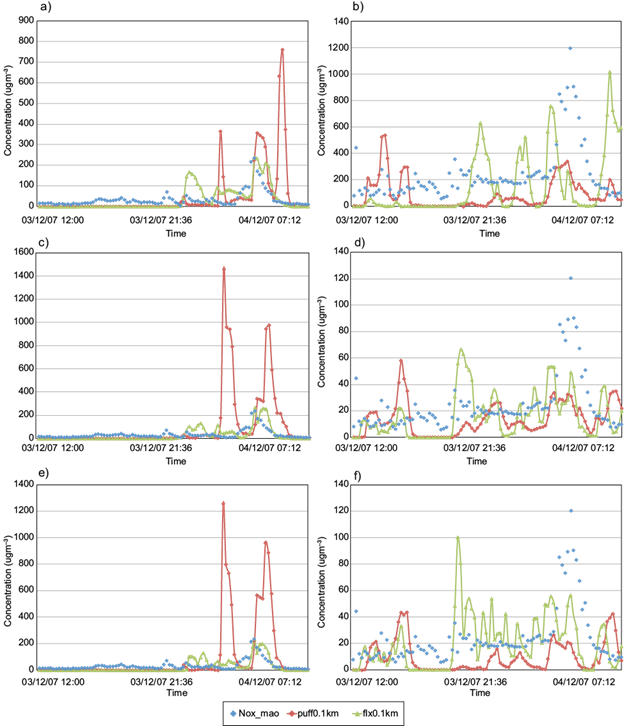
Fig. 7 Comparison between time series of 15-min NOx glc (µg m-3) observed (blue diamonds) at AQS1 station (a, c, e) and AQS2 station (b, d, f), and estimated with FLEXPART (green triangles line) and with CALPUFF (red diamonds line) at the same stations, along the simulation period: 16 UTC December 3 2007-16 UTC December 4 2007; using different meteorological grid resolution inputs: a, b: D4 (1 km); c, d: D5 (333 m); e, f: D6 (111 m).
In all simulations both models have similar tracer arrival time at both stations, that is, NOx glc first significant values started around 0 UTC December 4 at AQS1, and around 12 UTC December 3 at AQS2; although, from the observations time series, NOx seems to arrive earlier at AQS1, around 22 UTC December 3.
Considering the observed NOx glc peaks, the largest one in AQS2 (120 µg m-3) is observed at 07 UTC December 4. All simulations reproduce glc peaks around that time, but with lower values. This modeling peak underestimation occurs near primary road networks and at rush-hour traffic, so observed peaks seem linked to vehicle NOx emissions not taken into account in the models. The largest peak (below 80 μg m-3) is obtained in the flx1km simulation 2 h before the observed peak, while much lower peaks (below 60 μg m-3) are achieved at the observed peak time from the flx0.3km and flx0.1km simulations; also, the puff1km simulation achieves a significant peak at the same time as observed, but lower (below 40 μg m-3) than the other simulation peaks. In fact, both models get higher peaks several hours before the observed peaks, and these modelled peaks do not occur always at the same time for both models, even though the high sensitivity of plume transport to any errors in the wind direction provided by the WRF model is well known; also, the turbulent diffusion approaches applied for each model have a significant influence in these results.
As an example, in Figure 7a CALPUFF simulation obtains a significant glc peak at AQS1 at 4:15 UTC December 4; however, glc observations do not show any peak, in agreement with FLEXPART glc results. Otherwise, FLEXPART reproduces, in good agreement, the highest peak (200 µg m-3) observed in AQS1 at 5 UTC December 4, while all the CALPUFF simulations overestimate (close to 1 000 µg m-3) that observed peak.
3.2 Statistical evaluation results of NO x simulated concentrations
From the 15-min glc time series comparison some significant differences between observed and modeled ground-level concentrations arise. Therefore, statistics provide a quantitative estimation of model errors.
Table II shows the BOOT package statistical results obtained from FLEXPART and CALPUFF simulations results against observations at AQS1 and AQS2.
Table II BOOT statistics (µg m-3) for the simulation period, using FLEXPART and CALPUFF results against observations at AQS1 and AQS2 stations.
| Simulation | NMSE | FB | FBFN | FBFP |
| AQS1 Pointe-à-Pitre | ||||
| puff1km | 8.97 | -0.38 | 0.444 | 0.824 |
| flx1km | 1.79 | -0.050 | 0.459 | 0.509 |
| puff0.3km | 20.17 | -1.022 | 0.254 | 1.276 |
| flx0.3km | 1.89 | 0.093 | 0.540 | 0.447 |
| puff0.1km | 18.37 | -0.905 | 0.331 | 1.236 |
| flx0.1km | 1.60 | 0.232 | 0.605 | 0.373 |
| AQS2 Baie-Mahault | ||||
| puff1km | 2.86 | 0.913 | 1.034 | 0.121 |
| flx1km | 2.94 | 0.429 | 0.852 | 0.424 |
| puff0.3km | 1.76 | 0.558 | 0.749 | 0.191 |
| flx0.3km | 1.49 | 0.387 | 0.630 | 0.244 |
| puff0.1km | 3.41 | 0.870 | 1.061 | 0.191 |
| flx0.1km | 1.23 | 0.165 | 0.483 | 0.319 |
NMSE: normalized mean square error; FB; fractional bias; FBFN: underpredicting component of the FB; FBFP: overpredicting component of the FB.
From the core statistics, FB and RMSE better results were obtained using FLEXPART vs. CALPUFF, especially at AQS1, mainly because of the large CALPUFF glc peaks overestimations. Moreover, the higher meteorological resolution does not guarantee better CALPUFF results, with the worst results in puff0.3km at AQS1. However, using the FLEXPART flx0.1km simulation produced the best statistics at AQS1.
On the other hand, CALPUFF statistics are significantly better at AQS2 vs. AQS1, while FLEXPART statistics are similar at both stations. Also, the increase of meteorological resolution at AQS2 improves the FLEXPART results, with the minima NMSE and FB values from flx0.1km simulation. This effect is not always observed in CALPUFF results.
As expected, FBFP values show a pronounced overprediction of the observed concentrations at AQS1 in CALPUFF simulations, due to their too large modeled peaks. This FBFP overprediction of FB significantly exceeds the underprediction component FBFN. At the opposite, at AQS2 FBFN exceeds FBFP for both models’ simulations, that is, both models underestimate the observed concentrations along the simulation period. This shows that models results are extremely sensitive not only to the meteorological conditions (which are quite similar at both stations) but also to the station relative location from the emission source. Therefore, in the following sections other model comparisons and assessment approaches are also applied.
3.3 Spatial distribution of NO x
Considering previous statistics, the FLEXPART model performance using three different horizontal resolutions (1 km, 333 m, and 111 m) is better as the meteorological input grid resolution is finer. Therefore, as the clearest NOx glc spatial distribution, Figure 8 shows the models’ glc results over the 1-km horizontal resolution domain (D4). Compact isopleths with smooth contours from CALPUFF (Fig. 8a) and fragmented isopleths with irregular contours from FLEXPART (Fig. 8b) are observed. Particularly, the influence of two topographic tops at the west of the source is apparent in the fragmented FLEXPART glc distribution (not observed in the compact CALPUFF glc distribution).

Fig. 8 Spatial distribution of NOx (µg m-3) for the 1-km horizontal resolution domain (D4) at 05 UTC December 4, 2007 with source (red triangle) simulated with (a) CALPUFF and (b) FLEXPART. Also, the emission source (red triangle), the two air quality stations locations (red crosses), and topographic features are shown.
3.4 Plume impact evaluation from simulations
Plume impact evaluation based on the simulated maximum NOx glc, and Cmax over the simulation grid is shown in Figure 9, both for FLEXPART and CALPUFF at the three different grids resolutions. Unfortunately, it is not possible to estimate Cmax from glc observations for model assessment, because data from only two stations are available (Souto et al., 2014).

Fig. 9 Maximum NOx glc estimated with FLEXPART (green triangles) and with CALPUFF (red diamonds) for (a) 1-km; (b)-333 m, and (c) 111-m grid resolutions. The maximum simulated values for CALPUFF and FLEXPART are (a) 3321 and 716 µg m-3; (b) 12 925 and 2369 µg m-3, and (c) 20 133 and 2092 µg m-3, respectively.
For the NOx maximum glc, CALPUFF results are significantly higher than those from FLEXPART, and this difference increases with higher horizontal resolutions. These comparative results are consistent with the CALPUFF regulatory model condition, which guarantees glc overestimation in any condition. However, such large differences suggest that FLEXPART can be a better option for more accurate estimations in this complex domain if its systematic validation is performed.
Following the wind direction independent travel distance to the maximum concentration location (Xmax [Fig. 10]), FLEXPART estimates higher maximum distance values than CALPUFF, while minimum values are very similar. As Xmax maximum values usually correspond to unstable conditions, with higher PBL depth, these comparative results should be a consequence of the different PBL depth schemes applied to each model in unstable conditions. In addition, higher Xmax values from FLEXPART should produce a lower estimated NOx maximum value, as the plume has more time/travel distance to be dispersed. Also, glc values at the two air quality stations should be lower using FLEXPART, because the distances from the source to these station’s locations are lower than FLEXPART Xmax values, but similar to CALPUFF Xmax values. That is, these stations are located close to the CALPUFF maximum glc distance (Xmax) but before the FLEXPART Xmax. These differences can be related to the glc overestimation observed in the CALPUFF statistical assessment.

Fig. 10 Travel distance from the source to the maximum glc predicted with FLEXPART (green triangles) and with CALPUFF (red diamond). Grid resolutions: (a) 1 km, (b) 333 m, and (c) 111 m.
Besides, Xmax maximum values are higher with lower horizontal resolutions, both in FLEXPART and CALPUFF simulations; also, with differences between Xmax fluctuations over time, again depending on the resolution.
3.5 Spatial distribution of simulated maximum glc locations
The spatial distributions of estimated maximum glc locations using the CALPUFF and FLEXPART models are shown in Figure 11. CALPUFF simulations at three different horizontal resolutions show a reduced maximum impact area, close to the emission source and the air quality stations. This feature can produce high glc estimations at station locations, which justify the overestimation observed in the CALPUFF statistical assessment.

Fig. 11 Enlarged view of the maximum glc simulation locations using FLEXPART (+) and CALPUFF (x); also, the emission source (red triangle) and the two air quality stations (blue squares) locations are shown.
At the opposite, FLEXPART simulations produce different maximum impact areas than CALPUFF simulations using the same horizontal resolution. Also, FLEXPART maximum impact areas are different using different resolutions, as this model seems to be sensitive to the meteorological input horizontal resolution.
3.6 Simplified CALPUFF setup
The statistical assessment of the default CALPUFF setup, including original schemes for some features (as the transitional plume rise and the stack tip downwash) shows worse results than FLEXPART model results. However, for a better intercomparison between both models excluding these CALPUFF original schemes (not considered in the FLEXPART model), a second simplified CALPUFF setup is evaluated.
Table III shows the statistical results from BOOT software obtained from this second simplified CALPUFF setup simulations, compared to the observations at AQS1 and AQS2 stations.
Table III BOOT statistics (µg m-3) for the simulation period, using simplified CALPUFF simulations and observations at AQS1 and AQS2 stations.
| Simulation | NMSE | FB | FBFN | FBFP |
| AQS1 Pointe-à-Pitre | ||||
| puff1kmS | 5.50 | -0.240 | 0.448 | 0.688 |
| puff0.3kmS | 11.53 | -0.821 | 0.284 | 1.105 |
| puff0.1kmS | 11.39 | -0.581 | 0.397 | 0.978 |
| AQS2 Baie-Mahault | ||||
| puff1kmS | 5.30 | 1.317 | 1.335 | 0.018 |
| puff0.3kmS | 2.94 | 0.948 | 1.037 | 0.089 |
| puff0.1kmS | 7.83 | 1.382 | 1.434 | 0.052 |
NMSE: normalized mean square error; FB; fractional bias; FBFN: underpredicting component of the FB; FBFP: overpredicting component of the FB.
Although statistics show a poor CALPUFF performance as compared to the CALPUFF default setup simulations assessment (Table II), a significant improvement is observed. Therefore, original CALPUFF schemes for downwash of the plume rise and stack tip are not recommended in this case study. Otherwise, CALPUFF performance is still far from the FLEXPART statistics, as significant differences in model’s results remains.
4. Conclusions
Currently, two Lagrangian atmospheric dispersion approaches (particle and puff models) are usually applied to estimate passive pollutants dispersion over a complex terrain environment. In this work, a singular simulation domain, the Guadeloupe archipelago, was selected to test the FLEXPART Lagrangian particle model and the CALPUFF Lagrangian puff model. This domain includes several islands with complex terrain and strong sea influence in the Caribbean Region. Also, weak winds conditions were selected, as they produce the highest air pollution levels observed in this region. NOx emissions from a single power plant located on the main island were considered as a passive tracer.
Both Lagrangian models were coupled to the same WRF meteorological results at three different high-resolution grids (up to 111 m) to test their relative accuracy by comparison to 15-min ground level concentration observations at two air quality stations close to the emission source. During the testing period, the statistical model assessment showed that FLEXPART achieves significantly better agreement with glc observations than CALPUFF.
About the models’ intercomparison, the spatial distribution of NOx shows homogenous isopleths with smooth contours for CALPUFF, while fragmented isopleths with irregular contours are observed with FLEXPART, showing the effect of the complex topography over the NOx plume. Considering the estimated maximum NOx glc, CALPUFF results are much higher than FLEXPART, and CALPUFF results increase with the meteorological input resolution. Travel distance to the maximum glc is usually longer with FLEXPART than with CALPUFF, and further away from the air quality stations. This feature is in agreement with the higher CALPUFF maximum glc results and, also, its glc overestimation observed in this model assessment. Also, maximum glc locations from CALPUFF results are concentrated in a small area close to the air quality stations, while the corresponding FLEXPART locations are further away from the emission source and they extend over larger areas.

