


 text new page (beta)
 English (pdf)
 Article in xml format
 Article references
 Send this article by e-mail
 Cited by SciELO
  Similars in
SciELO
Similars in
SciELO 
 Permalink
1. Introduction
One of the main and most effective ways today to estimate air quality in an area is numerical prediction, which is a physical-mathematical tool that allows simulating pollutants transportation and dispersion in the atmosphere, as a result of the interaction between the meteorological conditions and those related with emission sources (Pu and Kalnay, 2019). This is done through air quality models, which are widely used to identify emission source contributions to atmospheric pollution problems; to assist in the design of strategies to reduce harmful air pollutants; to define the measurement systems location and resolution, and also to address their shortcomings in terms of spatial and temporal resolution. Once an air quality model is validated and adapted to the conditions of its area of application, it constitutes a representative, cheaper and faster option than measurements (Turtos, 2013).
Atmospheric dynamics are governed by physical laws expressed through mathematical equations that must be solved by the numerical models as an initial conditions problem integrated in time (Kalnay, 2003), which is a complex task that depends on the accuracy of a large number of internal and external parameters. Despite some advances in computer technology, initial data collection, numerical modeling techniques and model configurations (such as parameterizations or grid resolution), among others, evaluations of air quality models performance show that their solutions may still contain errors. In this sense, the most important topics include imperfect knowledge about the pollutants emissions pattern and rate, in addition to the chemical species initial and boundary conditions (Russell and Dennis, 2000).
From the first experiences in numerical prediction, particularly in air quality models, it became evident that one of the main limitations were the uncertainties in initial and boundary conditions, due to data scarcity and the use of inappropriate techniques to construct the model input grids (Charney, 1951). Today, numerical models use global and regional model outputs as the main input data, but these are often not representative of the study area or lack the necessary resolution. Therefore, there have been continued efforts to develop different tools that allow refining these data according to real observations.
Data assimilation is a powerful tool for this purpose. It can be defined as the process to include observed data in a model, maintaining the coherence of the laws that govern the evolution over time and the atmosphere physical properties (Bouttier and Courtier, 1999). Studies in this field consider data assimilation from different sources, such as surface observations, radiosondes, and indirect measurements obtained from radar and satellites, among others.
Data assimilation studies started from the numerical weather prediction when Richardson (1922) and later Charney et al. (1950) used available observations in manual interpolations to initialize a regular grid of points that would be digitalized, while its use in atmospheric chemistry is quite recent, because air quality models have been used routinely only since the mid-1990s (Bocquet et al., 2015). Elbern and Schmidt (2001) showed that optimizing initial conditions offered considerable improvement for ozone (O3) concentrations predicted in the atmosphere; similar conclusions were reached in other studies (Wu et al., 2008; Tombette et al., 2009; Wang et al., 2011; Curier et al., 2012), while Chai et al. (2006)) did it for nitrogen monoxide (NO), nitrogen dioxide (NO2) and polyacrylonitrile (PAN).
Approaches to data assimilation have also been used to combine measurements and model results in the air quality assessments context (Candiani et al., 2013), as well as to improve emission inventories (Mijling and van der A, 2012; Koohkan et al., 2013), to establish optimal monitoring networks (Rayner, 2004; Wu and Bocquet, 2010; Wu et al., 2010; Lauvaux et al., 2012), in inverse modeling to improve or identify errors in emission rates (Elbern et al., 2007; Vira and Sofiev, 2012; Yumimoto et al., 2012), for boundary conditions (Roustan and Bocquet, 2006), in the adjustment of model parameters (Barbu et al., 2009; Bocquet, 2012), and for satellite chemical variables data assimilation (Wang et al. 2011), among others (Bocquet et al., 2015).
Current challenges focus on coupled chemical-meteorological models because they offer the possibility to assimilate meteorological and chemical data. It is a more recent and less developed topic, although its use has increased in recent years employing a variety of techniques (Zhang, 2008; Baklanov et al., 2014; Bocquet et al. 2015). In this sense, several researches have been conducted with the coupled Weather Research and Forecasting Model with Chemistry (WRF-Chem): Pagowski et al. (2010) used Gridpoint Statistical Interpolation (GSI) and the Three-Dimensional Variational (3DVAR) method to assimilate both O3 and surface concentrations of particulate matter (PM) with a diameter of 2.5 µ or less (PM2.5) over North Americ; Liu et al. (2011) assimilated aerosol optical depth (AOD) from the Moderate Resolution Imaging Spectroradiometer (MODIS) to simulate a 2010 dust episode in Asia, while Chen et al. (2014) used a similar approach to improve simulations of PM2.5 and organic carbon surface concentrations during a wild biomass fire event in the United States; Pagowski and Grell (2012) compared 3DVAR and the Ensemble Kalman Filter (EnKF) techniques to assimilate PM2.5 surface concentrations; Schwartz et al. (2012) also used GSI and the 3DVAR technique to assimilate both AOD from MODIS and PM2.5 surface concentrations to improved simulated PM2.5 concentrations over North America, while Schwartz et al. (2014) assimilated the same data using the Ensemble Square Root Filter (EnSRF) and a hybrid ensemble 3DVAR methods; Jiang et al. (2013) also used GSI and 3DVAR to assimilate surface concentrations of PM with a diameter of 10 µ or less (PM10) in China; Peng et al. (2017) assimilated PM2.5 surface concentrations with EnKF, while Peng et al. (2018) also used EnKF to assimilate multi-species surface chemical observations, both to improve air quality forecasts over China, among others.
The above-mentioned papers only address the data assimilation of chemical variables. However, meteorology also plays a crucial role in air quality modeling, because it defines the physical and dynamical environment for atmospheric chemistry, that is, meteorology has a strong influence in the emissions transformation, chemical species, aerosols and PM in the atmosphere. In addition, the rates at which secondary species and aerosols form and certain chemical reaction take place are affected directly by relative humidity, solar energy, temperature, winds, and cover clouds. The significant uncertainty present in meteorological data during an air quality model simulation has the potential to affect negatively the simulation results. Therefore, as computer technology continues to rapidly grow and new remote sensing instruments become available, a greater amount of meteorological data can be collected and assimilated (with or without chemical data feedback) to improve air quality modeling (Seaman, 2000, 2003).
WRFDA is a data assimilation module developed for the Weather Research Forecast (WRF) model which allows to assimilate meteorological data. However, some research conducted by the National Center for Atmospheric Research (NCAR) is currently underway, focused on developing the WRFDA’s capacity to assimilate chemical data and to adapt this module for WRF-Chem. In this sense, Guerrette and Henze (2015) developed a new module based on WRFDA capable to assimilate both types of data using the Four-Dimensional Variational (4DVAR) technique, which was tested in a sensitivity study of anthropogenic and biomass burning sources in California. The main problem with this tool is that it has not yet been included in the WRFDA version available to the international scientific community (personal communication with the authors). In addition, Eltahan and Alahmadi (2019) showed the impact of meteorological data assimilation alone using both 3DVAR and 4DVAR algorithms within the WRFDA framework to simulate AOD of a dust storm over Egypt; they found out that assimilating wind speed data improved the model performance.
To the best of our knowledge, very little research related to data assimilation has been conducted in Mexico. In this sense, Bei et al. (2008) used the 3DVAR technique to assimilate meteorological fields such as wind, humidity and temperature to improve O3 simulations in Mexico City with the NCAR/Penn State mesoscale model (MM5) and the Comprehensive Air Quality Model with extension (CMAx). The best results were obtained early in the morning, especially regarding O3 concentration peaks and plume position. Based on this research, Bei et al. (2010) subsequently carried out meteorological data assimilation during the MCMA-2006/MILAGRO campaign (Molina et al., 2010) with similar objectives, but this time they used an ensemble forecast obtained from meteorological initial conditions, which were generated with the WRF-3DVAR technique (Barker et al., 2004). Then, following this same idea, Bei et al. (2012) investigated the uncertainties in the simulation of secondary organic aerosol in the Mexico City Metropolitan Area (MCMA) but using the WRF-Chem model also through ensemble simulations. In addition, Bei et al (2014) evaluated the impact of EnKF (Evensen, 1994) on air quality simulations in the California-Mexico border region during the Cal-Mex 2010 campaign and compared them with ensemble and nudging techniques.
This work aims to provide an initial overview of the influence on air quality numerical simulation with WRF-Chem over Central Mexico, of meteorological data assimilation from satellite observations and surface measurements using the 3DVAR algorithm. In addition, the WRFDA module was adapted to WRF-Chem. To carry out the simulations, an environmental contingency period between May 1 and 4, 2013 in the MCMA was selected. Six study cases were defined, taking into account the combination of two elements: the assimilated data sources and the numerical simulations start times. Firstly, a descriptive analysis of the assimilation process is performed. Then, the WRF-Chem model performance is evaluated for chemical and meteorological variables, using a set of statistical metrics that are proposed to determine which could be the most appropriate time to initialize the numerical simulation with meteorological data assimilation, as well as the best data source. In this way, a first approach to this topic is offered in Mexico, which can serve as a basis for future research about both meteorological and chemical data assimilation from different sources and is also applicable to other countries.
2. Materials and methods
2.1 Study area and modelling domains
The study area is located in the region known as central Mexico, which mainly includes Mexico City and the states of Mexico, Morelos, Hidalgo, Tlaxcala and Puebla (Fig. 1a). The most important region within this area is the MCMA, located in the Valley of Mexico basin, with geographic center in 19º 30’ N and 99º 02’ W. Its average height is 2240 masl. The MCMA is surrounded by elevations that allow pollutants accumulation over the city, imposing serious threats to human health and economic activities (SEMARNAT, 2002).
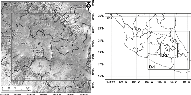
For all simulation runs, two modeling domains were constructed (Fig. 1b): a larger one (D-1) with 90 × 90 grid points and a 9-km resolution, and a smaller one (D-2) that covers the MCMA, with 88 ×88 grid points and a 3-km resolution. Both domains run at the same time and are completely interactive (two-way nesting). Vertically, 27 levels were considered.
2.2 WRF-Chem model: description and configuration
In this work we used the new generation regional air quality modeling system WRF-Chem (v. 3.8.1) developed by the National Oceanic and Atmospheric Administration Earth System Research Laboratory (NOAA/ESRL) and NCAR, to carry out the numerical simulations and to obtain hourly outputs. WRF-Chem simulates the emission, transport, mixing and chemical transformation of trace gases and aerosols simultaneously with the meteorology, i.e., both components are fully coupled and use the same transport scheme, the same horizontal and vertical grids, the same physics schemes and the same time-step for transport and vertical mixing. The model has several options for spatial discretization, diffusion, nesting, lateral boundary conditions and parameterization schemes for sub-grid scale physical processes. The physics consists of microphysics, cumulus convection, planetary boundary layer turbulence, land surface, longwave and shortwave radiation. WRF-Chem is used for investigating regional-scale air quality, field program analysis, cloud-scale interactions between clouds and chemistry, among others, and it also includes an initialization program to prepare the initial and boundary conditions for any domain, which is the Weather Preprocessing System (WPS) (Grell et al. 2005; Fast et al. 2006).
The physical parameterizations used in WRF-Chem were selected as follows:
The Yonsei University (YSU) scheme, a first-order non-local scheme with a counter-gradient term in the eddy-diffusion equation, was used for the planetary boundary layer (Hong and Dudhia, 2003).
The revised MM5-Similarity scheme, which uses a stability function to compute surface exchange coefficients for heat, moisture and momentum, was selected for surface layer (Zhang and Anthes, 1982).
The WRF Single-Moment class 5 (WSM5) scheme, which predicts five water species and allows mixed-phase cloud formation, was chosen as the microphysics option (Hong et al., 2004).
The Noah scheme (LSM), a four-layer model that calculates thermal and moisture stocks and fluxes on land, including vegetation, root and canopy effects, was used as soil-land parameterization (Chen and Dudhia, 2001).
Atmospheric short-wave and long-wave radiations were computed, respectively, by the MM5 Dudhia scheme, a simple broadband and downward solar flux scheme which uses look-up tables for cloud properties (Dudhia, 1989), and the Rapid Radiative Transfer Model (RRTM), which uses the correlated-k approach to calculate fluxes and heating rates efficiently and accurately (Mlawer et al., 1997).
The Kain-Fritsch scheme was used to represent cumulus. This scheme assumes that cloud base mass flux is determined by the amount of convective available potential energy in the environment that needs to be removed (Kain and Fritsch, 1993). Feedback from aerosols to the radiation scheme was turned on (aer_ra_feedback = 1) running with direct effect (cu_rad_feedback = .true), i.e., the shortwave and photolysis schemes included the effects of unresolved clouds in the simulations (Forkel et al., 2012).
The Regional Acid Deposition Model v. 2 (RADM2) was used as gas-phase chemistry mechanism. It determines the chemical species emissions distribution based on reactivity to the hydroxyl radical (OH) and includes 21 inorganic and 42 organic species with 136 chemical reactions (of which 21 are photochemical reactions) (Stockwell et al., 1990).
2.2.1 Input data
Meteorological data obtained from the North American Regional Reanalysis (NARR), developed by the National Centers for Environmental Prediction (NCEP), was used to generate the initial and boundary conditions of the meteorological fields for WRF-Chem. NARR is a long-term, dynamically consistent, high-resolution, high-frequency, atmospheric and land surface hydrology dataset. It provides data every 3 h and contains information of air temperature, zonal and meridional winds, pressure, geopotential height, humidity, soil data, precipitation and dozens of other parameters. The grid resolution is approximately 0.3º × 0.3º (32 km) with 29 pressure levels, covering the North American region (Mesinger et al., 2006).
In this work, we used the default chemical initial and boundary conditions hardcoded in the WRF-Chem model, based on an idealized, northern-hemispheric, mid-latitude, environmentally clean vertical profile from the NOAA Aeronomy Lab Regional Oxidant Model (NALROM) (Peckham et al., 2017). The anthropogenic emissions input was based on the 2008 Mexico National Emissions Inventory provided by the Secretaría de Medio Ambiente y Recursos Naturales (Ministry of the Environment and Natural Resources, SEMARNAT), which contains the classification of emissions from all fixed, mobile and area sources in their different categories and includes annual emissions by municipality of the main atmospheric pollutants such as sulfur dioxide (SO2), carbon monoxide (CO), NO, NO2, PM10, PM2.5, volatile organic compounds (VOCs), ammonia (NH3) and others (García et al., 2018). The Model of Emissions of Gases and Aerosols from Nature (MEGAN2; Guenther et al., 1994, 2006) was used to obtain biogenic emissions.
2.3 WRFDA data assimilation
WRFDA is a module implemented for the WRF which allows meteorological data assimilation through different techniques such as 3DVAR (Barker et al., 2004), 4DVAR (Huang et al., 2009), and hybrid variants that combine these with ensembles (Wang et al., 2008a, b). Variational techniques are applied through an iterative minimization process to a known cost function (the conjugate gradient is the iterative method implemented in WRFDA module), and one of its benefits is that dynamic constraints such as geostrophic and hydrostatic balances are included when the cost function is minimized. WRFDA allows the assimilation of conventional observation data in the American Standard Code for Information Interchange (ASCII) format using the observation processor (OBSPROC) tool, satellite radiance data in binary universal form for the representation of meteorological data (BUFR) and PREPBUFR format data (Barker et al., 2012).
The assimilation technique chosen to carry out the experiments was 3DVAR (Sasaki, 1970; Bouttier and Rabier, 1997), which can be described formally from an equation matrix for multiple grid points and variables, given by:
where J(x) is the Jacobian of x, which is a vector of n × m values (n is the number of points and m represents the dependent variables number); B and R are covariance matrices that contain statistical background and observation errors information, respectively; (x - x b ), known as analysis increments, is the subtraction between analysis x (field obtained after data assimilation) and first approximation field x b , known as background (initial condition obtained, in this work, from NARR fields); and x o represents observations, which are usually transformed into a consistent matrix with the system through a linear operator and are obtained in a 3-h window. In this way, from a control variable the minimum of J(x) is sought, looking for an analysis state as close as possible to the true state.
2.3.1 WRFDA for WRF-Chem
To adjust WRFDA for WRF-Chem it was necessary to turn off the model’s chemical component during the module compilation process. Once the executable for WRFDA was obtained, WRF-Chem was reinstalled in a directory underlying WRFDA. In this way, the model was ready to generate initial meteorological conditions with WRFDA and integrating them into WRF-Chem. For this, WRFDA requires three input files:
WRF first guess file, which is taken from WPS/real.exe output (wrfinput) for each assimilation cycle.
Observations, which include two sources provided by NCEP: a PREPBUFR data file (surface stations, ships, atmospheric soundings, GPS observations such as water vapor, and air traffic data), and BUFR satellite radiance data comprised by 10 polar satellite sensors (six advanced microwave sounding unit-A [AMSU-A] sensors from NOAA 15-16-18-19 Aqua Missions from the Earth Observing System [EOS-Aqua] and meteorological operational satellites-2 [METOP-2]; three microwave humidity sounder [MHS] sensors from NOAA 18-19 and METOP-2; and one atmospheric infrared sounder [AIRS] sensor from EOS-Aqua).
A background error statistics file provided by WRFDA using covariance option 3 (CV3) (Parrish and Derber, 1992).
For satellite radiance data assimilation it was necessary to make structural changes in the namelist.input file of the WRFDA module, such as to define the BUFR format as the type input data and to add detailed information about satellite sensors, among others. Moreover, to run WRFDA a script was written in which links to BUFR satellite radiance data, to PREPBUFR conventional observations data and the necessary coefficients for the Community Radiative Transfer Model (CRTM) were created. Finally, the data assimilation process was done witha 6-h cycling interval.
2.4 Study period and experiments description
To select the study period the dates of environmental contingencies reported in 2013 were taken into account. Therefore, the dates were set between May 1 and 4 because an air pollution contingency triggered by O3 began on May 2 at 17:00 LT lasting until the next day at 20:00 LT. Anomalous values of O3 concentrations were reported southwest of the MCMA, reaching a value in the Índice Metropolitano de Calidad del Aire (metropolitan index of air quality, IMECA) of 157 points. At the beginning of the study period the region was in a barometric marasmus. There was also a dry line to the north, which is typical during May within this region. In the last day of the period the study area was under a weak influence from migratory high pressures with weak gradients. In the center and south of the country, towards the Pacific coast, low pressures were observed.
The combination of two elements was taken into account to select the six case studies: the assimilated data sources and the numerical simulations start times. Three options were defined: without data assimilation (WA), with PREPBUFR data from NCEP assimilation (PB), and with PB plus satellite radiance data assimilation (PB+RD). Two start times were selected: May 1 at 00:00 UTC (19:00 LT) and May 1 at 12:00 UTC (19:00 LT) because they were synoptic times and had greater data availability.
2.5 Statistic metrics
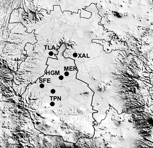
A statistical analysis for each proposed case was carried through point-by-point comparison between simulations results for three variables: temperature (T2), wind speed (WS) and O3 and observations from seven surface stations belonging to RAMA in the MCMA (Fig. 2): Hospital General (HGM), Merced (MER), Pedregal (PED), Santa Fe (SFE), Tlalnepantla (TLA), Tlalpan (TPN), and Xalostoc (XAL). These stations are deemed as suitable for the analysis of O3 behavior by the MCMA 2017 study framework (LTMCE2, 2017) and were available in the selected modeling period. The Unified Post Processor version 3.1 (UPPv3.1) and Model Evaluation Tool (METv5.0) release packages were used to perform this comparison.
The statistic metrics used to evaluate the model performance were the following:
Willmott Concordance Index (IOA; Willmott, 1981, 1982). This index is currently used as the main indicator for these purposes; it assesses the model performance on a scale from 0 to 1, where 1 is the perfect match with the measurement, and is calculated as:
Root Mean Square Error (RMSE; Fox, 1981): It describes the average difference between predictions and measurements, that is, the decrease of RMSE implies the improvement of the model performance, which can be defined as:
Pearson Correlation Coefficient (ρ; Pielke, 1984): It describes the level of agreement between forecast and observed values, and is defined as:
Normalized Bias (BIAS; Pielke, 1984): It indicates whether there is a model overestimation or sub-estimation with respect to the measurements, which can be calculated as:
where p i is the predicted value; o i is the value observed at the same time i; o̅ is the average of observed values; p̅ is the average of predicted values; N is the measurements number per station, and σ is the standard deviation.
3. Results and discussion
3.1 Initial conditions performance in the assimilation process
First of all, we calculated analysis increments since they provide measures for the variation of variables once the minimization process is done. WS and T2 are taken as examples of this, because they are part of the modified meteorological fields in the data assimilation process. All results are shown for the D-2 domain.
Figures 3 and 4 show (a) a first approximation to T2 and (b-c) analysis fields and their (d-e) increments fields, obtained for the two different assimilation cases defined (PB and PB+RD) and the two chosen time test cases (00:00 and 12:00 UTC). The background fields show a generally warm environment in all domain for both times, with higher T2 values than the normal averages for May, which is in agreement with the presence of high pressures in the area, which was mentioned above. However, considerably high T2 values are observed in the extreme relief area (valley and mountain), indicating that the initial conditions without data assimilation, which would be used to perform the simulation, might not show the T2 actual behavior in the study area.
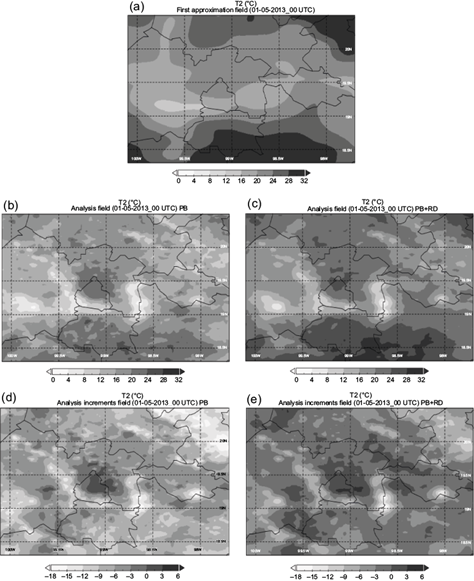
Fig. 3 (a) T2 first approximation, (b, c) analysis and (d, e) increments fields for PB and PB+RD cases at 00:00 UTC.
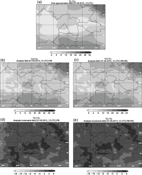
Fig. 4 (a) T2 first approximation, (b, c) analysis and (d, e) increments fields for PB and PB+RD cases at 12:00 UTC.
The analysis fields indicate that both data assimilation options modify T2 values throughout the domain, which shows their impact on the variable. Also, through the increment fields it is observed that, in general, data assimilation aims to decrease T2 initial values in a large portion of the domain, which is of order 0(10) in accordance to the characteristic scale of the studied variable, reaching even more than -18 ºC over mountain areas at 00:00 UTC. This shows that the original data from NARR (which are average analysis fields for variables) seem unable to describe T2 values in this relief type; however, by including observations data in the assimilation process, they can correct T2 initial fields. For the MCMA, both assimilation options indicate that a positive correction should be made to T2 variables greater than 3º C, which are very frequent in urban areas highly affected by the urban heat island (UHI) effect, a phenomenon that numerical models cannot simulate efficiently.
On the other hand, at 00:00 UTC it is observed that the PB+RD case suggests a less abrupt T2 values correction compared to the PB option, which could be explained because PB+RD includes satellite radiance data assimilation that have full coverage of the study area and allow a data correction that best describes the real variable behavior, while PREPBUFR is mainly composed of stations data and PB suggests more abrupt corrections. However, at 12:00 UTC the differences between corrections proposed by both assimilation options are much smaller, which may be related to the fact that there is a greater volume of meteorological data available at this time; therefore, point observations can improve their effectiveness.
Figures 5 and 6 show the wind fields (wind direction [WD] and WS) following the same idea as the previous two figures. In general, the backgrounds for both periods indicate a continuous wind flow with variable direction (prevailing from the west and southwest) over the domain, although for the southern MCMA winds are observed from the northwest at 12:00 UTC. No wind patterns are identified through the images at the synoptic or mesoscale scale. The smoothness in the WS and WD initial fields is appreciated, which is related to the fact that NARR offers average fields for the different variables reflecting their characteristics on a larger scale than that used in the modeling domain mesh in this research, and this may not accurately describe the variable behavior in the study area.
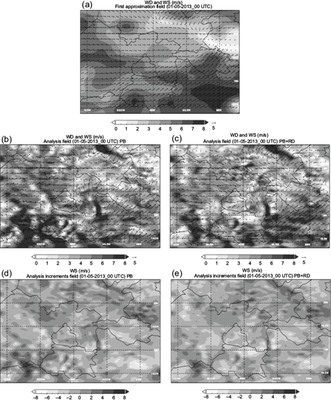
Fig. 5 (a) WS first approximation, (b, c) analysis and (d, e) increments fields for PB and PB+RD cases at 00:00 UTC.
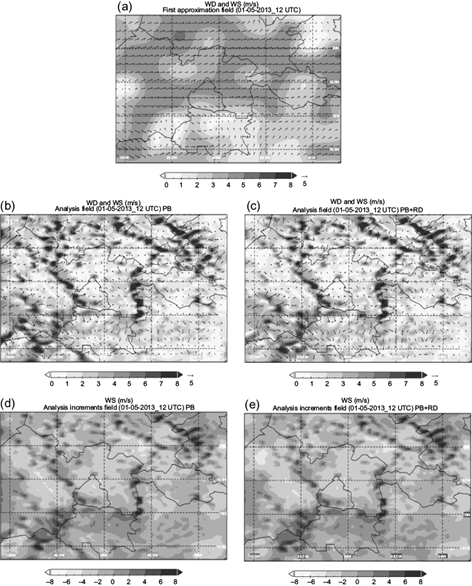
Fig. 6 (a) WS first approximation, (b, c) analysis and (d, e) increments fields for PB and PB+RD cases at 12:00 UTC.
When assimilation is performed, analysis fields show changes in WD and WS for all cases (highest at 12:00 UTC) for the entire domain, with much more irregular variables’ behavior, which would be more in line with the terrain characteristics in the area and with the grid resolution used for the simulations. This could improve the description of pollutants dispersion over the study area, given the decisive influence of the wind over it.
The pattern obtained for increment fields at 12:00 UTC is very similar for both assimilation options. However, the most notable differences are observed at 00:00 UTC, which again may be related to the greater data availability at 12:00 UTC; also, it should be noted that satellite radiance data assimilation has less influence for WD and WS than for T2.
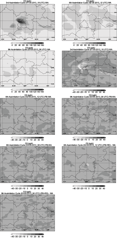
Figures 7 and 8 represent temporal evolution of the T2 and WS spatial distribution (a-c), respectively, analysis increments for PB (d-f) and PB+RD cases (g-i) for the 3rd, 6th and 9th assimilation cycles (starting from 00:00 UTC). These graphs show that the T2 and WS fields undergo changes during the different cycles indicated for each assimilation case and also with respect to the others. For both variables, the absolute values of the increments are much lower in each cycle than in the first case analyzed in Figures 5 and 6, which may be due to the “cold start way” in which the data assimilation process begins. This means that the analysis fields from NARR were used to obtain the initial conditions for the first assimilation cycle for t = 0, which may cause the greatest increment differences to be observed in the initial cycle. On the other hand, the rest of the cycles begin in a “warm start way”, that is, the immediate previous WRF-Chem model forecast is taken as an initial condition to carry out the next assimilation cycle. Therefore, analysis increments are expected to be smaller since the forecast is the numerical integration result over time of all the equations in the model, taking into account the initial conditions previously adjusted; this should reflect a better variables’ behavior in relation to the case study being modeled with respect to the domain spatial resolution, topography and specific physical processes. Furthermore, as the time-steps run increase, the numerical model itself adjusts continuously, therefore analysis increments should decrease as assimilation cycles increase.
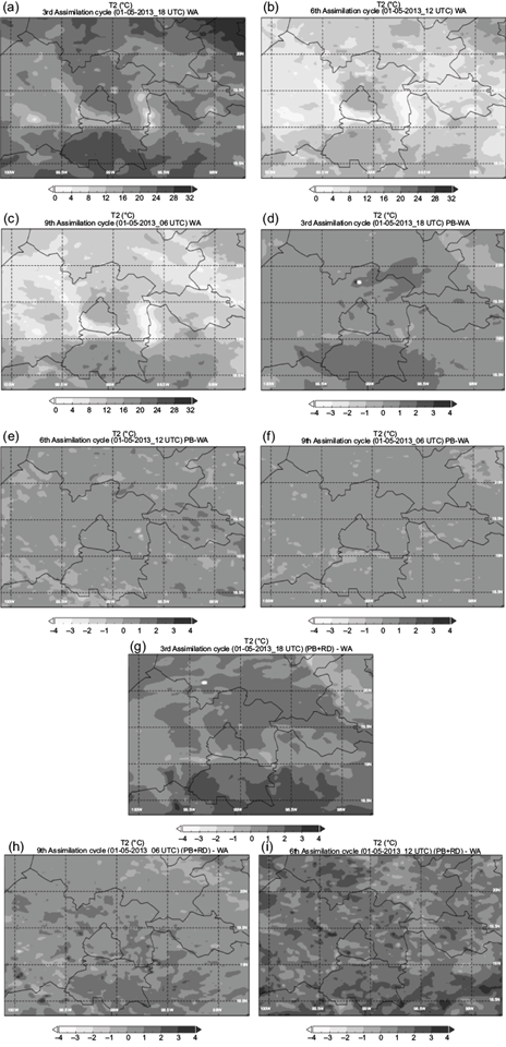
Fig. 7 (a-c) Temporal evolution of the T2 spatial distribution, (d-f) analysis increments for PB cases, and (g-i) analysis increments for PB+RD cases, for the 3rd, 6th and 9th assimilation cycles (starting from 00:00 UTC).
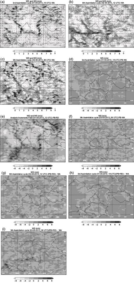
Fig. 8 (a-c) Temporal evolution of the WS spatial distribution, (d-f) analysis increments for PB cases, and (g-i) analysis increments for PB+RD cases, for the 3rd, 6th and 9th assimilation cycles (starting from 00:00 UTC).
For T2, the largest increases (up to 4 ºC) are attained in the 6th assimilation cycle for the PB+RD case, while for WS the increments proposed are smaller, and they are also greater in the PB+RD option with respect to PB.
It is now possible to appreciate the importance of data assimilation (mainly satellite radiance) to obtain useful T2 and WS initial fields for numerical simulation at higher resolutions than data models such as NARR, which allows to show the real behavior of variables in the study area and to contribute positively to the improvement of model performance.
Figure 9 shows the temporal evolution of the O3 spatial distribution (a-c) and the differences between O3 fields with respect to the WA field for PB (d-f) and PB+RD (g-i) for the 3rd, 6th and 9th assimilation cycles (starting from 00:00 UTC). It can be observed through the differences between these fields (which are not analysis increments because this variable was not assimilated) that changes in the O3 values do occur throughout the domain, both when comparing the assimilation options between each other and with respect to the WA case, also with the course of assimilation cycles. These differences do not exceed more than 40 ppb and are generally concentrated in the MCMA and surrounding areas. The highest values are observed in the PB+RD case. Therefore, it is worth noting how O3 varies both in time and space once the meteorological data have been assimilated, which shows that there is a sensitivity (although low) in the chemical variables’ behavior when meteorological initial conditions are modified.
3.2 Statistical analysis
The statistical analysis results obtained for each proposed case are presented below.
Figures 10 and 11 show, respectively, the times series for observed and modeled T2 and WS values in (a, d) all stations, (b, e) MER, and (c, f) SFE at 00:00 and 12:00 UTC for all assimilation cases. The time elapsed since the data assimilation starting time is indicated in the x axis. Figure 10 shows that the model is capable of reproducing the T2 daily cycle reaching maximum and minimum values at the corresponding times. Nevertheless, the maximum is underestimated in all cases, which is very frequent in air quality simulations due to the UHI effect in the MCMA (Jáuregui, 1997; Cui and de Foy, 2012). Furthermore, the PB+RD option is closest to the observed values, mainly at 12:00 UTC, as depicted in the MER and SFE graphs. It is observed that modeled cases are closer to observations at the times in which the assimilation is carried out. On the other hand, Figure 11 shows that the WS behavior is not as accurate as T2, although modeled values of this variable are closer to observations. Both for all stations and for the individual stations MER and SFE, better results are attained at 00:00 UTC, especially during the first steps of execution. PB+RD is the assimilation source that shows best results for WS.
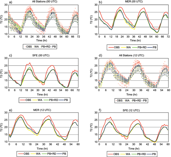
Fig. 10 Time series for simulated and observed T2 values over (a, d) all stations, (b, e) MER and (c, f) SFE at 00:00 and 12:00 UTC for all assimilation cases.
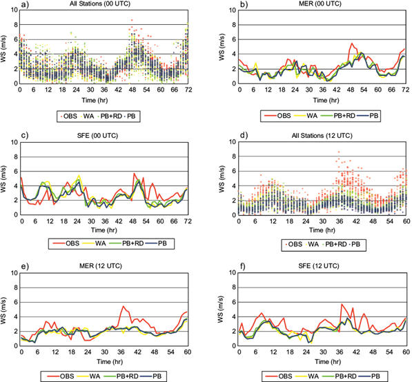
Fig. 11 Time series for simulated and observed WS values over (a, d) all stations, (b, e) MER and (c, f) SFE at 00:00 and 12:00 UTC for all assimilation cases.
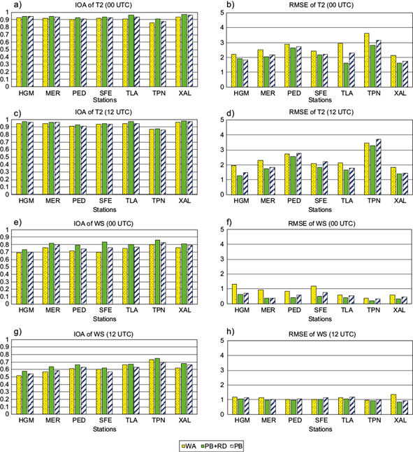
Fig. 12 IOA and RMSE indicators for T2 and WS for each selected station and all assimilation cases at 00:00 and 12:00 UTC.
Figure 12 shows the IOA and RSME indicators for T2 and WS for the seven selected stations and for all assimilation cases at 00:00 and 12:00 UTC. The obtained results converge with those mentioned in Figures 10 and 11. Regarding the T2 variable, IOA values greater than 0.9 are observed for all stations in each case and time, which means there is a good agreement between modeled and observed values. The PB+RD option has the highest IOA in six of the seven stations at 00:00 UTC and in all stations at 12:00 UTC. Also, RMSE values for T2 are always between 1 and 3 ºC, with the lowest values found at 12:00, and TPN being the lowest performing station. It should be noted that except for one case, PB+RD has the lowest RMSE values, which confirms it is the best assimilation source. In the case of WS, IOA statigraphs show best results at 00:00 UTC, with values always greater than 0.7 for PB and PB+RD, which are suitable values for WS. PB+RD values remain above 0.8 most of the time, while WA permanently exhibits the worst performance with lower IOA values. The best performing station is, paradoxically, TPN, which did not perform optimally for T2, while the station with greater differences regarding observations is HGM at 12:00 UTC. RMSE values for WS are always lower than 1.5 m s-1, which is an optimal result for WS, a variable that is commonly difficult to model. These RMSE values are better at 00:00 UTC and with PB+RD source.
Figure 13 displays the temporal evolution of simulated and observed O3 concentrations, while Figure 14 depicts the IOA and RSME indicators for O3 concentrations, both for all selected stations and specifically MER and SFE at 00:00 and 12:00 UTC, including all assimilation cases. Overall, the model represents adequately the daily O3 cycle, although the correspondence between modeled and observed values is not as remarkable as in the case of meteorological variables. It is shown that the model is capable of approaching the variables’ maximum at both times, but it tends to overestimate minimum values. Besides, the overall performance for each assimilation case source is different from that shown for T2 and WS. For example, although PB+RD exhibits the best results, it can be seen that in some time series intervals values obtained from the modeling of WA are closer to observations, while PB always exhibits a lower performance. On the other hand, the results shown in the MER and SFE stations are very contrasting. The O3 temporal series in MER shows adequate values while in SFE a rather poor performance is observed. The values of IOA and RMSE show an acceptable agreement between model and measurements. In the case of IOA at 00:00 UTC, six of the seven stations have values greater than 0.7, which is a good result for this variable. Also, the best results are observed for all stations beginning data assimilation at 12:00 UTC, with higher IOA values. For RMSE, all values are around 30 ppb. PB has again the lower performance, while PB+RD continues to be the best assimilation source.
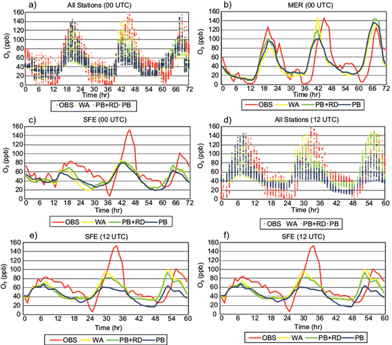
Fig. 13 Time series for simulated and observed O3 concentrations over (a, d) all stations (b, e), MER and (c, f) SFE at 00:00 and 12:00 UTC for all assimilation cases.
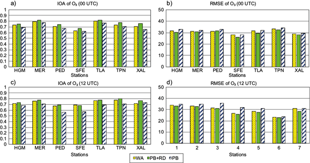
Fig. 14 IOA and RMSE indicators for O3 concentrations for each selected station and all assimilation cases at 00:00 and 12:00 UTC.
In addition, Table I shows the statigraphs average values found for all stations, both at 00:00 and 12:00 UTC and for all assimilation options, which allows to observe the general trends for each studied variable. For T2, the metrics results for both schedules are similar and appropriate for this variable. The best performance is obtained with PB+RD at 12:00 UTC. BIAS indicates that, compared to observations, the model underestimates values in all cases. RMSE is always lower than 2.5 ºC and ρ and IOA are always greater than 0.9. For the WS case, a better performance is observed for PB+RD at 00:00 UTC. The IOA and ρ values at 00:00 UTC are greater than 0.7 in all cases, while for 12:00 UTC values are less than 0.66 and 0.63, respectively. These are generally good results for this variable, although they could be better, especially at 12:00 UTC. BIAS indicates that the model tends to slightly overestimates the values as compared to observations. For O3, the best performance is achieved by the PB+RD option at 12:00 UTC, with ρ between 0.6 and 0.7, IOA always greater than 0.67 and RMSE between 25 and 30 ppb, which are suitable values for this variable. BIAS indicates that, compared to observed values, the model underestimates O3 concentrations for all selected stations.
Table I IOA, BIAS, RMSE and ρ values for T2, WS and O3 concentrations regarding the WA, PB and PB+RD assimilation cases at 00:00 and 12:00 UTC.
| 00:00 UTC | 12:00 UTC | ||||||
| WA | PB | PB+RD | WA | PB | PB+RD | ||
| T2 | IOA | 0.91 | 0.93 | 0.94 | 0.93 | 0.94 | 0.95 |
| BIAS | -2.33 | -1.94 | -1.62 | -1.76 | -1.30 | -1.28 | |
| RMSE | 2.49 | 2.41 | 2.32 | 2.46 | 2.24 | 2.22 | |
| ρ | 0.93 | 0.94 | 0.96 | 0.95 | 0.95 | 0.96 | |
| WS | IOA | 0.75 | 0.77 | 0.80 | 0.64 | 0.63 | 0.66 |
| BIAS | 0.02 | -0.03 | -0.05 | 0.07 | 0.13 | 0.05 | |
| RMSE | 0.83 | 0.54 | 0.40 | 1.19 | 1.21 | 1.18 | |
| ρ | 0.72 | 0.76 | 0.79 | 0.61 | 0.59 | 0.63 | |
| O3 | IOA | 0.71 | 0.67 | 0.72 | 0.72 | 0.68 | 0.74 |
| BIAS | -9.61 | -11.56 | -8.57 | -8.74 | -10.65 | -7.95 | |
| RMSE | 27.71 | 29.98 | 26.39 | 26.94 | 29.44 | 25.53 | |
| ρ | 0.65 | 0.62 | 0.67 | 0.64 | 0.64 | 0.68 | |
4. Conclusions
In order to test the influence of meteorological data assimilation on air quality modeling within the MCMA, the WRFDA data assimilation module is adapted to the WRF-Chem model. BUFR satellite radiance and PREPBUFR data from NCEP are assimilated at 00:00 and 12:00 UTC, using the 3DVAR algorithm. Six sensitivity cases were analyzed for an environmental contingency reported between May 1 and 4, 2013, in the MCMA, to determine the best possible combination including assimilated data sources and the starting time of numerical simulations.
From the increments calculated in the analysis, we obtained a variation measure undergone by the T2 and WS initial fields once the minimization process was carried out. This variation also allows to show if the new fields obtained through data assimilation better represent the behavior of meteorological variables and describe the physical processes within the study domain, mainly related to the grid resolution. In this sense, we obtained that the increment of these values decreases as the assimilation cycles increase, which is in line with the use of a cold start for the initial step and a warm start for the following time steps, as well as the model's own adjustment through the different simulation time steps. In addition, these increment values increase by schedules when more data is available.
The statistical results show that meteorological data assimilation has a positive influence in values obtained with the WRF-Chem model for related variables such as T2, indicating there is a good agreement between modeled and observed data, with IOA values greater than 0.90 for all the study cases. The model originally tends to underestimate T2 values, which is evidenced by the negative BIAS values observed in WA. This is somehow corrected through data assimilation, reaching a BIAS value of -1.28 for the PB+RD case at 12:00 UTC, which overall is the best combination for the T2 variable. An improvement is also observed in the WS fields, mainly for the PB+RD case at 00:00 UTC, although not in the same magnitude as for the T2 field. RMSE and BIAS values are close to 0 for the mentioned option, demonstrating the positive influence of data assimilation, with IOA and ρ values greater than 0.75 and 0.70, respectively. At 12:00 UTC, lower results were obtained.
Regarding the influence of meteorological data assimilation on the chemical variables, changes in the behavior of O3 are observed after running the simulation, in correspondence with the results obtained by Bei et al. (2010, 2012), Liu et al. (2017) and Mizzi (2017). The metrics analyzed indicate a slight improvement for the PB+RD case, while in general PB values show larger differences in the WRF-Chem model performance. Also, the best results are achieved with runs starting at 12:00 UTC, which may be related to the largest volume of surface observations data available at that time. The best data source is PB+RD, which exhibits the benefits provided by satellite radiance data assimilation, mainly for T2.
Therefore, chemical data assimilation (instead of meteorological data) using 3DVAR and other techniques, such as 4DVAR or EnKF, are proposed as a first step to improve estimates of pollutant concentrations obtained from air quality modeling with WRF-Chem in the MCMA. Better results are obtained by constantly improving assimilation of the initial chemical conditions, through less uncertain emissions database used in the simulations.

