


 nueva página del texto (beta)
 Inglés (pdf)
 Artículo en XML
 Referencias del artículo
 Enviar artículo por email
 Citado por SciELO
  Similares en
SciELO
Similares en
SciELO 
 Permalink
1. Introduction
Determining crop water requirements is important in irrigation. Crop water requirements are a function of the reference crop evapotranspiration (ET 0 ). Crop evapotranspiration is basically estimated using ET 0 and the crop coefficient (Kc). The Penman-Monteith equation (PM) has performed better than other methods for estimating ET 0 , therefore, it has been recommended as the international standard for calculating this value based on meteorological data (Allen et al., 1998; Ozturk and Apaydin, 1998). The fact that a large volume of data is needed to utilize the PM equation complicates its use, as databases can be incomplete. Recording data may require large storage space (Ditthakit and Chinnarasri, 2012). Evaporation pans have been found suitable for estimating ET 0 ; hence, for determining crop water requirements. They constitute a widely used technique due to their simplicity and low cost (Ozturk and Apaydin, 1998; Raghuwanshi and Wallender, 1998; Irmak et al., 2002; Ditthakit and Chinnarasri, 2012). Various types of evaporation pans are used; however, class A and sunken Colorado pans are the most common. ET 0 is dependent on the measured pan evaporation and pan coefficient (K p ). Values of K p for class A and sunken Colorado pans, under various plant covers and environmental and climatic conditions are presented as tables in FAO-24 (Doorenbos and Pruitt, 1977) and FAO-56 (Allen et al., 1998). However, when observed conditions are out of the range listed in the tables, estimates of K p values may lead to errors. Frevert et al. (1983), Cuenca (1989), Snyder (1992), Allen et al. (1998), Raghuwanshi and Wallender (1998) and Grismer et al. (2002) developed regression models to determine K p based on data from class A pans. Allen et al. (1998) and Abdel-Wahed and Snyder (2008) modeled K p with data from class A pans in arid regions having dry surfaces. The modified Snyder approach has shown the largest errors; however, as compared to other approaches, it resulted in smaller errors. This study, conducted in the Amol region of Iran, reported the accuracy of a number of methods for calculating K c (Zare et al., 2011).
Machine learning algorithms have been successfully used for ET 0 simulation. Torres et al. (2011) estimated ET 0 in the first stage of an irrigation project in central Utah. In the second stage, they used historical meteorological parameters to simulate ET 0 with the help of the estimated parameters. They used the multivariate relevance vector machine (MVRVM) in both stages. The proposed method was tested in terms of robustness and stability with bootstrap analysis. Shrestha and Shukla (2015) successfully applied support vector machine for the modeling of ET using hydroclimatic variables in a subtropical environment based on six years lysimeter data. The results showed that the proposed model can be used in the development of region-specific K c to improve ET c estimates. Feng et al. (2017) applied extreme learning machine (ELM) and generalized regression neural networks (GRNN) to daily ET 0 simulation only with temperature data in the Sichuan basin (southwest China). The results showed that temperature-based GRNN and ELM models are appropriate alternatives for the accurate simulation of ET 0 . Dou and Yang (2018) simulated daily ET 0 values in four different ecosystems using flux tower observed data with ELM and the adaptive neuro-fuzzy inference system (ANFIS). They compared the results of these two methods with the results of the artificial neural network and support vector machine methods. The proposed models generally achieved best performance in forest ecosystems, and worst in cropland ecosystems. Granata (2019) applied the M5P regression tree, bagging, random forest, and support vector regression to simulate ET 0 in central Florida, characterized by a humid subtropical climate, and emphasized that machine learning algorithms may be a powerful tool for the prediction of actual evapotranspiration when a time series is available. Granata et al. (2020) simulated daily ET 0 based on climatic variables such as net solar radiation, depth to water, wind speed (WS), mean relative humidity (RH), and maximum, minimum, and mean temperatures, using random forest, additive regression of decision stump, multilayer perceptron, and k-nearest neighbors algorithms. They found that random forest and k-nearest neighbors provide slightly better performance than additive regression of decision stump and multilayer perceptron.
Data mining techniques, like the M5 model tree, have been applied to many problems in hydrologic engineering, water science and environment. M5 model trees were used to model monthly reference ET 0 (Sattari et al., 2013a); to predict daily reference evapotranspiration in Bonab (Sattari et al., 2013b) and monthly precipitation in northwest Iran (Sattari et al., 2014); to determine possible drought periods in Ankara (Sattari et al., 2012), and for pan evaporation modeling (Kisi, 2015). Ditthakit and Chinnarasri (2011, 2012) applied neural networks and the M5 tree model to determine class A and sunken Colorado pan coefficients and found more accurate estimates of K p than with other methods. Class A pans are widely used in Iran (Zare et al., 2010).
Agriculture and food availability are of vital importance to the Iranian economy and its citizens. Large areas in East Azerbaijan are devoted to the growth of onions, tomatoes, potatoes and wheat, but this region has an annual average precipitation of 297 mm and a semi-arid climate; therefore, it is necessary to effectively utilize the limited water resources available.
The amount of evaporation, which is very important in the hydrological cycle, negatively affects agricultural water management in arid regions. It is critical to determine the plant water consumption easily and accurately (which depends on evaporation and the K p value) in order to plan and operate irrigation systems. There are many equations and methods for the calculation of reference evapotranspiration; however, since different hypotheses and meteorological data are used for these methods, different results may be obtained at regional level (Grismer et al., 2002). There are no agricultural stations in the study area that adequately measure meteorological parameters. The equalities used in evapotranspiration calculations do not give consistent results due to the lack of data, instruments and equipment in the existing stations (Ditthakit and Chinnarasri, 2012). In this research, the M5 decision tree and the FAO methods are used to determine daily class A pan coefficients in replacement of tables or regression equations, in a dry fallow land at four different stations located in the province of East Azerbaijan under cold and dry climate.
2. Materials and methods
2.1 Study area
Data from four meteorological stations located in Ahar (Vardin and Sattarkhan dam), Sarab (Mirkooh), and Mianeh (Shahryar dam), East Azarbaijan, were used in this study (Fig. 1). East Azerbaijan is one of the 31 provinces of Iran, covering an area of approximately 47 830 km² with a population of around four million people. Its economy is based on the heavy and food industries, agriculture, and handicraft. Grains, fruits, cotton, rice, nuts, and tobacco are the staple crops of the region. The climate of East Azerbaijan is affected by the Mediterranean continental climate and a cold semi-arid climate. Gentle breezes off the Caspian Sea have some influence on the climate of the low-lying areas. Data required for calculating daily pan coefficients, including air RH and WS, as well as the expertise for installing the pan, were provided by the East Azerbaijan Regional Water Company. The stations specifications are listed in Table I.
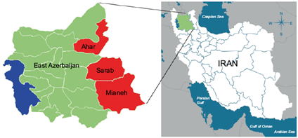
Table I Description of the four stations.
| Windward side distance (m) | P (mm) | Tmean (ºC) | Number of data | Geographical information | Station name | ||
| Elevation (m) | Latitude | Longitude | |||||
| 12 | 403.1 | 9.35 | 2863 | 1837 | 38º 00′ | 47º 30′ | Sarab, Mirkouh |
| 15 | 339.7 | 11.34 | 2508 | 1400 | 38º 26′ | 46º 59′ | Ahar, Vardin |
| 15 | 365.8 | 11.06 | 731 | 1415 | 38º 27′ | 46º 55′ | Ahar, Sattarkhan dam |
| 16 | 277.6 | 15.45 | 2127 | 1015 | 37º 30′ | 48º 03′ | Mianeh, Shahryar dam |
Class A pans are used at these stations to measure evaporation. They have been installed in fallow land surrounded by green vegetative cover (the best practice for installing pans). The daily pan coefficients were obtained using a previously developed table (Table II) and available data. These parameters were used as inputs for the model.
Table II Values of the class A pan coefficients (K p ) at different pan locations, mean relative humidity and wind speed
| Case B: Pan placed at dry fallow area Rh mean (%) | Case A: Pan placed at short green cropped area Rh mean (%) | Windward side distance of green crop (m) |
Wind speed (m s-1) |
||||
| high > 70 | medium 40-70 | low < 40 | high > 70 | medium 40-70 | low < 40 | ||
| 0.85 | 0.80 | 0.70 | 0.75 | 0.65 | 0.55 | 1 | Light < 2 |
| 0.80 | 0.70 | 0.60 | 0.85 | 0.75 | 0.65 | 10 | |
| 0.75 | 0.65 | 0.55 | 0.85 | 0.80 | 0.70 | 100 | |
| 0.70 | 0.60 | 0.50 | 0.85 | 0.85 | 0.75 | 1000 | |
| 0.80 | 0.75 | 0.65 | 0.65 | 0.60 | 0.50 | 1 | Moderate 2-5 |
| 0.70 | 0.65 | 0.55 | 0.75 | 0.70 | 0.60 | 10 | |
| 0.65 | 0.60 | 0.50 | 0.80 | 0.75 | 0.65 | 100 | |
| 0.60 | 0.55 | 0.45 | 0.80 | 0.80 | 0.70 | 1000 | |
| 0.70 | 0.65 | 0.60 | 0.60 | 0.50 | 0.45 | 1 | Strong 5-8 |
| 0.65 | 0.55 | 0.50 | 0.65 | 0.60 | 0.55 | 10 | |
| 0.60 | 0.50 | 0.45 | 0.70 | 0.65 | 0.60 | 100 | |
| 0.55 | 0.45 | 0.40 | 0.75 | 0.70 | 0.65 | 1000 | |
| 0.65 | 0.60 | 0.50 | 0.50 | 0.45 | 0.40 | 1 | Very strong > 8 |
| 0.55 | 0.50 | 0.45 | 0.60 | 0.55 | 0.45 | 10 | |
| 0.50 | 0.45 | 0.40 | 0.65 | 0.60 | 0.50 | 100 | |
| 0.45 | 0.40 | 0.35 | 0.65 | 0.60 | 0.55 | 1000 | |
Source: Doorenbos and Pruitt, 1977; Allen et al., 1998.
2.2 Evaporation pans
Evaporation from an open water surface can be easily measured with evaporation pans. If there is no precipitation, water that evaporates over a time period (mm day-1) equals the reduction in water depth during the same time period. Pans are used to measure the combined effects of radiation, wind, and humidity within the region on evaporation from open water surfaces. Pan evaporation has the following relation with the reference crop evapotranspiration:
where ET 0 is the reference crop evapotranspiration (mm day-1), K p is the pan coefficient (dimensionless), and ET p is the pan evaporation (mm day-1).
The selection of K p is dependent on the type of pan along with the plant cover at the station, conditions around the pan, wind conditions, and air RH. Besides the installation expertise of a pan, the surrounding environment impacts the evaporation measurement. This impact is particularly important when the pan is installed in a fallow land. Two general installation practices were considered: (1) the pan was installed in a land with short green plant cover but surrounded by fallow land, and (2) the pan was installed at fallow land surrounded by green plant cover. The values of class A pan coefficients from FAO 56 (Allen et al., 1998) are shown in Table II.
Instead of using Table II, regression Eqs. (2) and (3) derived by Allen et al. (1998) were used to determine K p :
where K p is the pan coefficient, U 2 is the average daily WS at 2 m height (m s-1), RH is the average daily RH (%), and F is the fetch or distance of the identified surface type upwind of the evaporation pan (grass or short green agricultural crop for case A, dry crop or bare soil for case B). In order to use these equations, U 2 must be between 1 and 8 m s-1, RH between 30 and 84%, and fetch distance between 1 and 1000 m. A local adjustment is required to determine K p if either the table or the regression equation are used. Allen et al. (1998) recommended that the use of tables or the corresponding equations may not be sufficient to consider all local environmental factors influencing K p . Therefore, local adjustments may be required.
2.3 M5 regression tree and performance evaluation
Machine learning, data mining and decision trees are artificial intelligence methods which have been very popular during the last few decades. Many sub-methods have been developed and applied to water resources management. The M5 decision tree model was introduced by Quinlan (1992); thereafter it has been widely used in data mining, which refers to the process of discovering patterns in data. It is widely used as a classification and prediction model. A decision tree algorithm produces a model in the form of a tree. It is essentially a model where linear regression equations at the leaves replace terminal class values (Pal, 2006; Coria et al., 2016). Decision tree models are easy to understand and include root, branches, nodes, and leaves. They are usually constructed from top to bottom and the last branch ends with a leaf. Each node is associated with a specific attribute, whereas branches represent ranges of values. A predictive variable performs a splitting function. Split ranges are selected to minimize errors at each node (Quinlan, 1992). The first step in building a decision-tree model is to use a splitting criterion. In the M5 algorithm, this criterion is based on entropy, which measures the amount of disorder in data. The error of the model is usually assessed by measuring the accuracy in predicting target values of unseen cases (Alberg et al., 2012).
The splitting process is iterated at each node until the final node (leaf) is reached, where the total of the square deviations about the mean approaches zero. A decision-tree might be rather large; thus, to reduce its size, branches can be pruned to produce a manageable tree. There are two pruning methods: (1) pre-pruning: before the tree reaches its maximum size, and (2) post-pruning: after the tree reaches its maximum size. In the first method, the pruning process does not allow for the production of extra branches; however, in the second method, the pruning is performed after the tree attains its maximum growth.
After pruning, a smoothing process takes place to compensate for sharp discontinuities that inevitably happen between adjacent linear models at the leaves of the pruned tree. This is especially the case for models constructed from a smaller number of samples (Alberg et al., 2012).
In this research, the WEKA software (Eibe, 2016), developed at the University of Waikato in New Zealand was used to predict pan coefficients using the M5 model. It is the leading open-source software in the field of artificial intelligence. Studies in this field are not just about providing input data to the software; many alternatives need to be carefully examined to find the best model. The data was divided into four different training (consisting of 66, 70, 75 and 80% of the original data) and testing sets. The performance of the models developed in the study was evaluated based on the root mean square error (RMSE), coefficients of determination (R2), the unpaired two-sample t-test and the Nash-Sutcliffe efficiency (NSE) index.
3. Results and discussion
The FAO method was used in this study to determine daily pan coefficients in fallow land at all four stations. Values of K p calculated via the traditional method were used as target variables. RH, WS at 2 m above ground surface, and windward side distance (fetch) to the green crop were considered as independent variables. Table III shows the specifications of the statistical data at each station. Note that the Sarab, Ahar Vardin and Ahar Sattarkhan stations have an average WS of 1.41-1.91 m s-1, while WS at Mianeh is only 1.1 m s-1. Average RH values in each of the four stations range from 60.7 to 64.5%; however, the average K p value was determined as 0.8 in the Sarab station, whereas in Ahar Vardin, Ahar Sattarkhan and Mianeh these values were very close to each other: 0.7, 0.71 and 0.71, respectively. The highest calculated K p value was 0.8 and the lowest 0.45, with the Sarab station displaying the largest range.
Table III Values of pan coefficients and independent variables at the four stations.
| Station | Statistics | Wind speed (m s-1) | Relative humidity (%) | Pan coefficient |
| Sarab, Mirkouh | Maximum | 6.50 | 100 | 0.80 |
| Minimum | 0.28 | 10.5 | 0.49 | |
| Mean | 1.41 | 60.7 | 0.80 | |
| Standard deviation | 0.58 | 18.5 | 0.07 | |
| Ahar, Vardin | Maximum | 8.24 | 84 | 0.80 |
| Minimum | 0.90 | 30 | 0.45 | |
| Mean | 1.91 | 61.7 | 0.70 | |
| Standard deviation | 1.01 | 14.0 | 0.06 | |
| Ahar, Sattarkhan dam | Maximum | 7.00 | 95.5 | 0.80 |
| Minimum | 0.25 | 23.5 | 0.54 | |
| Mean | 1.65 | 64.5 | 0.71 | |
| Standard deviation | 1.01 | 12.2 | 0.05 | |
| Mianeh, Shahriar dam | Maximum | 3.81 | 82.5 | 0.80 |
| Minimum | 0.45 | 44.0 | 0.64 | |
| Mean | 1.10 | 61.0 | 0.71 | |
| Standard deviation | 0.47 | 8.7 | 0.04 |
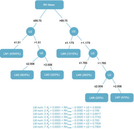
As an example, Figure 2 exhibits the M5 decision-tree model for the Shahriar dam station. Seven linear relations computed via the M5 decision-tree model were introduced in Figure 2, namely K p , mean RH, and WS at 2 m above the ground surface. Since daily input data were used to construct the model, daily calculations were also made for K p . As seen in Figure 2, K p values can be calculated easily by using seven simple linear equations considering the change in only mean RH and WS at 2 m above the ground surface. These parameters are available for all regions or can be obtained by simple observations. Thus, K p values can be simulated at a low cost without highly trained specialists, and can significantly contribute to agricultural activities. For example, the tree diagram in Figure 2 for the Shahriar dam station in Mianeh shows that if the mean daily RH is ≤ 69.75%, and daily WS at 2 m above the ground surface is 1.51 m s-1, the daily pan coefficient will be calculated using the linear relation LM num 1 (K p = 0.0001 × RHmean - 0.0007 × U2 + 0.6926).
As seen in Table I, the Mianeh station only has data for 733 days, while the Ahar Sattarkhan station has data for 2863 days. Four different training datasets were tested in this study because of these differences in length. These data sets consist of 66, 70, 75 and 80% of the original data. Four different linear model sets, coefficient of determination and RMSE were computed for each station. The preferred model is marked in bold letters in Table IV. As it may be seen in this table, the best decision tree model is based on 80% of the data from the Sattarkhan dam station in Ahar (with 2863 data records). With this data percentage, we simulated the pan coefficient with R2 = 0.9916 and RMSE = 0.0049 using 16 linear relations.
Table IV Daily results generated by the M5 decision tree model for all stations under numerous scenarios.
| Station | Number of data | Training data (%) | Number of linear models | R2 | RMSE |
| Ahar Sattarkhan dam | 2863 | 66 | 16 | 0.9912 | 0.0050 |
| 70 | 16 | 0.9916 | 0.0050 | ||
| 75 | 16 | 0.9916 | 0.0050 | ||
| 80 | 16 | 0.9916 | 0.0049 | ||
| Ahar Vardin | 2508 | 66 | 13 | 0.9914 | 0.0059 |
| 70 | 13 | 0.9926 | 0.0056 | ||
| 75 | 13 | 0.9944 | 0.0049 | ||
| 80 | 13 | 0.9952 | 0.0045 | ||
| Mianeh Shahriar dam | 731 | 66 | 7 | 0.9936 | 0.0044 |
| 70 | 7 | 0.9936 | 0.0041 | ||
| 75 | 7 | 0.9936 | 0.0043 | ||
| 80 | 7 | 0.9937 | 0.0042 | ||
| Sarab Mirkouh | 2127 | 66 | 13 | 0.9926 | 0.0059 |
| 70 | 13 | 0.9931 | 0.0058 | ||
| 75 | 13 | 0.9930 | 0.0059 | ||
| 80 | 13 | 0.9922 | 0.0060 |
Note: values in bold letters show the best results.
At the Vardin station in Ahar (with a total of 2508 records), when 80% of the data was allocated to training, the M5 decision tree was able to model pan coefficients using 13 linear relations with R2 = 0.9952 and RMSE = 0.0045. At the Shahriar dam station in Mianeh (731 records), when 70% of the data was allocated to training, the M5 decision tree model was able to model pan coefficients using seven linear relations with R2 = 0.9937 and RMSE = 0.0042. At the Mirkouh station in Sarab (2127 records), when 70% of the dataset was allocated to training, the M5 decision tree was able to model pan coefficients using 13 linear relations with R2 = 0.9931 and RMSE = 0.0058. Quite interestingly, neither the coefficient of determination nor the RMSE improved when the size of the training data increased at the Sarab station. However, at the other three stations, R2 increased as the training data size increased and RMSE decreased. At the Sarab station, the best result was obtained with 70% of the records. The decrease in the number of data points and the number of linear models at the Mianeh station did not adversely affect the M5 tree results.
Dispersion diagrams of the pan coefficients determined by the FAO method and the decision tree models in each station are shown in Figure 3, indicating that the decision tree accurately simulates the pan coefficient at each station. The coefficient of determination is larger than 0.99 for all stations (0.9916-0.9952).

Fig. 3 Scatter diagrams of the pan coefficients estimated by the FAO method and by the decision tree model.
Time series of simulated and observed monthly mean pan coefficients for each station are shown in Figure 4. At the Vardin station, the M5 tree model simulated the higher K p value in only four out of 16 months of testing. K p values remain the same for 12 months. In the Sattarkhan station, the K p value remained higher during four of 19 test months, whilst it remained lower during five months. In the Mirkouh station, the M5 tree model simulated higher K p values during five of the 21 test months and lower in only one month. At the Shahriar station, the M5 tree model simulated lower values in all seven test months.
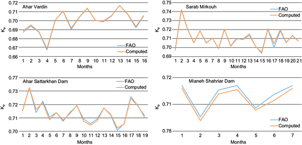
Fig. 4 Time series of the monthly pan coefficients estimated by the FAO method and the decision tree model.
As shown in Table V, the unpaired two-sample t-test was applied, and NSE and skewness were calculated to determine the best model for each station during the test period. T is simply the calculated difference represented in units of standard error. The greater the magnitude of T, the greater the evidence against the null hypothesis. This means there is a greater evidence of having a significant difference. As T tends to 0 the absence of a significant difference is more likely. The P value is used to accept or reject the null hypothesis. The lowest P value was 0.722 in Mianeh and the highest was 0.96 in Sattarkhan. It was concluded that there was no statistically significant difference between the calculated K p and the K p value simulated with the M5 model for all stations. A similar situation arises when NSE values (from 0.989 to 0.994) are examined.
Table V Results of the unpaired two-sample t-test, the Nash-Sutcliffe efficiency index and skewness for the test period.
| Station | t-test T and P values | Nash-Sutcliffe efficiency index | Skewness |
| Sarab, Mirkouh | -0.10/0.917 | 0.993 | -0.1826 |
| Ahar, Vardin | -0.16/0.873 | 0.994 | 0.0422 |
| Ahar, Sattarkhan dam | 0.05/0.960 | 0.991 | 0.5394 |
| Mianeh, Shahryar dam | 0.36/0.722 | 0.989 | 1.4100 |
4. Conclusions
In this paper an easy and feasible method to determine the amount of ET 0 (crop water requirement) using data obtained from an evaporation pan, is presented. Evaporation pans can be easily installed by farmers in all climatic conditions. Measurements can be made by them, and the required amount of irrigation can be calculated without the need for expertise (Ditthakit and Chinnarasri, 2012). The K p value plays a key role in the ET 0 calculation. If the K p value is determined correctly, ET 0 and the crop water requirements can be calculated, enabling effective irrigation planning and optimum use of agricultural water. Predicting ET 0 and consequently estimating the crop water requirements is of great importance in irrigation water management. Evaporation pans are useful to determine ET 0 in regions without full meteorological stations and data. So, the pan coefficient is considered a key parameter for estimating ET 0 in irrigation practices. In this research, the FAO-24 and FAO-56 class A pan equation was used to calculate K p . RH and WS values, as well as the windward side distance (fetch) of the green crop, were considered as inputs to the decision tree model for estimating the pan coefficient.
Four different training datasets, consisting of 66, 70, 75 and 80% of the original data were tested in this study. The average RH for all stations ranged from 60.7 to 64.5%, whereas the WS varied between 1.1 and 1.91 m s-1. Moreover, K p values ranged from 0.7 to 0.8.
A total of 49 simple linear relations were obtained via the M5 decision tree model for each of the four stations to compute the K p value. The best results were obtained when 70% of the data were used for training in the Mirkouh station, and 80% at the other stations. At this stage, R2 values ranged between 0.9916 and 0.9952, and RMSE values from 0.0042 to 0.0058. No linear relationship was found between R2 and RMSE values at the Sarab station. Moreover, the unpaired two-sample t-test and the NSE were also calculated in our research. P values ranged from 0.722 to 0.96 whereas NSE values renged from 0.989 to 0.994.
Results show that the decision tree model is able to accurately predict K p at all four stations in the relatively cold and arid study area. Therefore, this model can be used in arid climates, with the resulting linear equations being simple, understandable, and easy to apply.
The most important finding in this study is an easier method to estimate K p with a number of linear functions obtained via the M5 model from RH and WS, without the need of complex tables and equations. Ditthakit and Chinnarasri (2011) estimated K p values with a non-linear genetic artificial intelligence method (R = 0.99). In our study, K p was estimated with the same accuracy but with easier linear equations from the M5 model. Finally, the estimation of K p can help calculating ET 0 more accurately, leading to effective irrigation planning. The only limitation of this study is that it was conducted in a specific region of Iran and the results are not applicable to regions with different climates. Our suggestion is to perform similar studies in regions with different climatic conditions.

