


 text new page (beta)
 English (pdf)
 Article in xml format
 Article references
 Send this article by e-mail
 Cited by SciELO
  Similars in
SciELO
Similars in
SciELO 
 Permalink
1. Introduction
Extreme climate events (ECE) must be periodically monitored and analyzed in detail, due to their role as high impact agents on society, environment, and ecosystems. An extreme climatic or meteorological event refers to the occurrence of a climatic or meteorological variable which value is above or below a threshold that is close to the upper (or lower) limits of the range of observed values of the variable (Seneviratne et al., 2012). ECE are important because of their impacts, but they are difficult to quantify statistically, as they are infrequent and occur at multiple scales (Palmer and Räisänen, 2002). The definitions of “rare” vary, but an ECE would normally be as rare as, or rarer than, the 10th or 90th percentile of the observed probability density function.
It is likely that different ECE affect specific regions and increases in their frequency and intensity have been detected in several regions of the world (Brown et al., 2008; Almazroui et al., 2014; Chen et al., 2015; Wypych et al., 2017; Caloiero, 2017). It is expected that these ECE will intensify in the future in response to global climate changes caused by the emission of greenhouse gases (Beniston et al., 2007; Gao et al., 2012; Lau and Nath, 2012; Easterling et al., 2016; Grotjahn et al., 2016; Schoof and Robeson, 2016).
There are basically two fundamental approaches to study ECE: global circulation models (GCMs), and statistical models using the extreme value theory (EVT). Contemporary GCMs, such as those used for the 5th Coupled Model Intercomparison Project (Taylor et al., 2012) are a key component of regional climate change projections, but their limited spatial resolution reduces their utility in estimating local or regional extremes without substantial post-processing (Schoof and Robeson, 2016). On the other hand, the central issue of EVT is the modeling of extreme events, and the main purpose of this theory is to provide asymptotic models for the distribution tails (Furió and Meneu, 2011). Therefore, EVT aims at deriving a probability distribution of events at the far end of the upper or lower ranges of the probability distributions (Coles, 2001); its main advantage is that it allows for estimating and analyzing the probability of occurrence of events that are outside of the observed data range (Raggad, 2018).
For these reasons, EVT is the approach that has been chosen in this research due to its wide applicability in different fields that are related to extreme weather and climate events and their impact: ecology (Moritz, 1997; Meehl et al., 2000; Dixon et al., 2005; Katz et al., 2005; Jentsch et al., 2007; Burgman et al., 2012); extreme temperatures and heat waves (Meehl and Tebaldi, 2004; Della-Marta et al., 2007; Parey et al., 2007; García-Cueto et al., 2010; Waylen et al., 2012; Tanarhte et al., 2015; Liu et al., 2015; Shen et al., 2016); extreme rainfall (Katz et al., 2002; Koutsoyiannis, 2004; Friederichs, 2010; Papalexiou and Koutsoyiannis, 2013; Kim et al., 2015; Boucefiane and Meddi, 2019); and damages to the communities that affect agroecosystems through changes in soil moisture and evapotranspiration rates (Miralles et al., 2014; Whan et al., 2015; Guan et al., 2015; Hatfield and Prueger, 2015).
Changes in extremes of temperature and precipitation have been evaluated in different regions of the world. However, until the Fourth Assessment Report of the Intergovernmental Panel on Climate Change (Trenberth et al., 2007), the cities had been treated as “noise-generating” entities in globally studied climatic signals. In the Fifth Assessment Report of the Intergovernmental Panel on Climate Change (IPCC, 2013), a special chapter was dedicated to the subject of cities, and their role in climate change. This is not surprising, as although cities are very important contributors to social and economic well-being, they require an uninterrupted source of energy for all their activities. Cities consume approximately 75% of global primary energy and emit between 50-60% of the greenhouse gases (GHG) on the planet (Rosenzweig et al., 2011). This figure can be raised to 80% when indirect emissions generated by inhabitants of the cities are included (UN-Habitat, 2011; Kraussmann et al., 2017). Thus, cities promote global warming, and contribute to an increase in average surface temperature at the planetary level.
In addition to the global effects of GHG, the worldwide upward trend of urban growth must be considered, both in population and in its areal extension. This growth has generated environmental problems, not only air pollution and solid waste, but also those concerning a different environmental product, such as the genesis of an urban climate. In particular, the main connotation of urban climate is the formation of an urban heat island, which in turn requires additional water and energy to maintain thermal comfort through air-conditioned spaces (Coutts et al., 2012; Wang et al., 2016; de Munck et al., 2018, Skelhorn et al., 2018). Thus, cities that are already particularly vulnerable to ECE caused by global climate change must now also consider the effects caused by local climate change. Therefore, it can be inferred that because a city is the geographical space that brings together a majority of the population and provision of services, it will be where the greatest vulnerabilities associated with the impacts of climate change manifest themselves (UN-Habitat, 2011).
In Mexico approximately three out of four people (72.3%) live in cities according to Fundación Centro de Investigación y Documentación de la Casa and Sociedad Hipotecaria Federal (CIDOC-SHF, 2011). This percentage is expected to increase in the medium term, as according to projections of the National Population Council the number of people in 384 localities of the National Urban System will increase by 16.6 million (from 82.6 million in 2010 to 99.3 million in 2030) as a result of an annual average growth rate of 0.92% (Hernández et al., 2014). The urban proportion of the national population will increase to 77.9% (18.1 million new urban inhabitants). This trend of the geographic dynamics of cities is inequitable with low levels of quality of life and urban sustainability, and not all cities have the same development potential. Thus, the challenges in facing climatic risks such as heat waves and floods will be massive if quantitative scientific studies are not carried out.
Very little research has been conducted in Mexico on extreme climate values in urban environments (Magaña et al. 2003, 2012; Cavazos and Rivas, 2004; Ríos-Alejandro, 2011; García-Cueto et al., 2013, 2014, 2018; Martínez-Austria and Bandala, 2017). This can be explained by a limited access to measured climate data, limitations in the geographical coverage of the networks of stations, and interruptions in climate series due to missing data. In view of this and given the quantitative uncertainty of the climate extremes mentioned at the urban level and their great importance for the assessment of risks and adaptation proposals, this study selects some cities in Mexico with important increases in population and in areal extension, which have recently been affectated by ECE.
Thus, this study has three main objectives: (a) to detect thermal behavior in some growing cities of Mexico, (b) to model extreme temperatures through the EVT, and (c) to make projections of return levels for extreme temperatures in a future changing climate.
This paper is organized as follows: section 2 presents the climatology of extreme values in Mexico; section 3 presents the study area and the climate data, and section 4 provides a theoretical outline of the methodology. The results and discussion are presented in section 5. In section 6, conclusions are drawn.
2. Climatology of extreme temperature values of Mexico
Figures 1 and 2 show the 10th and 90th percentiles of minimum and maximum temperatures, respectively (Cavazos et al., 2013), for the period 1961-2000; the methodology used in these figures is described in Colorado-Ruiz et al. (2018). According to extreme climate indices derived from reliability ensemble averaging (REA) (Fig. 1), the coldest winters and their 10th percentile (P10) during the winter months of December, January, and February (DJF) for Mexico are characterized by minimum temperatures below 0 ºC in the highlands of the Sierra Madre Occidental and the Mexican High Plateau, and between 0 and 5 ºC in much of northern Mexico. Figure 2 shows that the extreme values of the 90th percentile (P90) of the maximum temperatures during the summer months of June, July, and August (JJA) expand the area covered by the isotherms of 25 and 40 ºC to a narrower strip in the border region. This region of semiarid climate is the most extreme in Mexico; therefore, it is the most susceptible to negative impacts caused by increases in temperature.
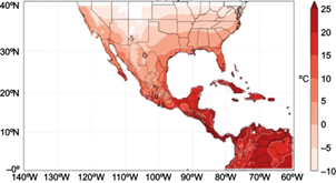
Fig. 1 Thresholds of P10 of minimum temperature for winter, obtained with the ensemble of the Reliability Ensemble Averaging (REA) for 1961-2000 (Cavazos et al., 2013).
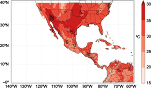
Fig. 2 Thresholds of P90 of maximum temperature for summer, obtained with the ensemble of the Reliability Ensemble Averaging (REA) for 1961-2000 (Cavazos et al., 2013).
The projected climate changes at a national level (Cavazos et al., 2013) agree with those obtained globally (Alexander et al., 2006; Caesar et al., 2011; Song et al., 2014). Regarding those related to the increase in the frequency of heat days, heatwaves and variability in precipitation will exacerbate problems related to natural and human systems (Ummenhofer and Meehl, 2017). If we analyze the 10th and 90th percentiles of extreme temperatures at the national level, there is a notable lack of reliable and timely information at the regional and urban levels for risk assessment, which justifies the study carried out herein.
3. Data and study area
A digital historical collection of daily temperature data for several cities in Mexico was possible using information from climatological stations operated by the Servicio Meteorológico Nacional (SMN, National Weather Service). Unfortunately, the selection of urban areas of interest faced some limitations, as not all climate stations have the same record length, and none had a strict data quality control. Based on a previous analysis of the growth of some cities in Mexico and the occurrence of climatic events that have affected them in important ways, 21 cities were selected in the first instance. However, an analysis of the quality of climate information limited the study to only 12 cities. These cities are heterogeneously distributed in the country because, as mentioned above, they were selected for their population growth and urban development. Data quality control was carried out for the daily information for each city, consisting of the following synthetic process.
The SMN database from the Climate Computing Project (CLICOM) was extracted in the .csv format, using Matlab and RClimdex software. The climatic information was explored, and quality control was performed for the original database. The daily meteorological values of maximum temperature (TXX) and minimum temperature (TNN) were selected with a computation routine; at the same time, a continuity of the time series was sought by adding missing dates and values, if possible, and adding a -99.99 label for missing data. Subsequently, the database was imported into the RClimdex program (Zhang and Yang, 2004), ensuring the internal and temporal consistency of the daily climatological information. This quality control validated the following: (1) internal coherence, by verifying that the maximum temperature was always greater than the minimum temperature; (2) identification of atypical values and changes in the seasonal cycle or variability of the data through visual inspection of the time series of TXX and TNN, and (3) identification of values located more than four standard deviations (σ) from the mean as outliers and possible errors. Finally, outliers were verified individually to determine if they had been caused by an atypical event or if the measurement was incorrect and had to be discarded.
Temporal homogeneity of the data was then evaluated using the RHtest V3 software (Wang and Feng, 2010) to identify abrupt jumps or change-points. This homogeneity test is based on a two-phase regression model with a linear trend for the entire series, applied to selected series for each of the cities.
The final selection included the following cities and/or intra-urban regions for the detailed analysis of extreme temperatures: Aguascalientes, Mexicali, Tijuana, Tuxtla Gutiérrez, Mexico City (with analysis of the climatological stations of Úrsula Coapa, Gran Canal, and Milpa Alta), León, Guadalajara, Monterrey, Puebla, Tlaxcala, Veracruz and the metropolitan area of the Valley of Mexico, including the urban areas of Toluca, Aculco and Chapingo (Table I). Their locations are presented in Figure 3 and, as can be seen, the analysis includes cities distributed in central Mexico (18-25º N latitude), a city in southeastern Mexico (Tuxtla Gutiérrez), another in northeastern Mexico (Monterrey), and two more in northwestern Mexico (Tijuana and Mexicali).
Table I City or urban region, climatological station number, elevation, period of useful data, historical values of extreme maximum temperature, and extreme minimum temperature.
| ID | City or urban region | Climatological station numbera | Elevation (masl) | Period | TXX (ºC) | TNN (ºC) |
| 1 | Aguascalientes | 01030 | 1889 | 1950-2015 | 40.0 | -6.0 |
| 2 | Mexicali | 02033 | 4 | 1950-2012 | 52.0 | -7.0 |
| 3 | Tijuana | 02038 | 120 | 1950-2012 | 45.0 | 0.0 |
| 4 | Tuxtla Gutiérrez | 07165 | 570 | 1980-2010 | 42.0 | 7.1 |
| 5 | Úrsula Coapa, CDMX | 09014 | 2256 | 1971-2013 | 34.5 | -3.0 |
| 6 | Gran Canal, CDMX | 09029 | 2239 | 1952-2008 | 38.5 | -7.5 |
| 7 | Milpa Alta, CDMX | 09032 | 2420 | 1963-2012 | 34.0 | -2.5 |
| 8 | León | 11095 | 1828 | 1959-2014 | 39.5 | -2.5 |
| 9 | Guadalajara | 14066 | 1550 | 1957-2013 | 47.0 | -1.5 |
| 10 | Aculco, ZMVM | 15002 | 2490 | 1970-2011 | 32.0 | -5.0 |
| 11 | Toluca, ZMVM | 15126 | 2726 | 1974-2009 | 33.6 | -10.0 |
| 12 | Chapingo, ZMVM | 15170 | 2250 | 1954-2010 | 37.5 | -8.5 |
| 13 | Monterrey | 19049 | 495 | 1949-2009 | 48.0 | -7.5 |
| 14 | Puebla | 21035 | 2122 | 1955-2013 | 36.5 | -6.0 |
| 15 | Tlaxcala | 29030 | 2230 | 1969-2013 | 39.2 | -7.4 |
| 16 | Veracruz | 30192 | 16 | 1930-2014 | 42.7 | 7.9 |
aClimatological station number refers to the key that the National Weather Service (SMN) of Mexico manages in its files.
TXX: extreme maximum temperature; TNN: extreme minimum temperature; CDMX: Mexico City; ZMVM: metropolitan area of the Valley of Mexico.

Our study focused on ECE using a parametric non-stationary generalized extreme value (GEV) distribution model, which tacitly assumes that extreme events are changing over time as climate changes. Instead of the climate change indices used in García-Cueto et al. (2018), the current study directly applies extreme temperature values. In addition, the non-stationary GEV model is applied to investigate how the return levels of extreme temperatures might change in the future.
It is worth mentioning that for the city of Mexicali, due to the importance of extreme temperatures for human comfort and energy consumption for use in air conditioning, other studies have been carried out (García-Cueto et al., 2010, 2013). Unlike current research, in García-Cueto et al. (2010) warm days were modeled with the GEV and the maximum temperature was included as a covariate, without performing a temporal trend analysis of extreme temperatures. Their difference with respect to García-Cueto et al. (2013) is that the trends of extreme temperatures and their return periods are updated with a methodological process that requires a re-parameterization of the GEV model, which gives greater reliability in its estimation.
4. Methodology
In this section we present the techniques used for trend analysis and a brief review of the GEV distribution, to provide a basis for the modeling of extreme temperature events. As described in section 1, the GEV distribution is used to model extremes in atmospheric science and in many other scientific fields. Using the trends of annual temperature series, we describe the non-stationary models, the criteria for deciding which GEV model to use, the estimation of the parameters of the GEV distribution, and the return levels.
4.1 Trend analysis
The detections of monotonic trends of increase or decrease in TXX and TNN in a time series were analyzed using the Mann-Kendall non-parametric test (Mann, 1945; Kendall, 1975) and Sen’s method for slope estimates (Sen, 1968). The Mann-Kendall test is based on ranges and has been found to be an excellent tool for detecting trends in climatic applications (Burn and Hag Elnur, 2002; Mugume et al., 2016). One of the advantages of this test is that the data does not need to be adjusted to any distribution. The second advantage of this test is its low sensitivity to sudden breaks owing to non-homogeneous time series, extreme values (outliers), and non-linear trends (Helsel and Hirsch, 1992; Tabari et al., 2011). Given its robustness, the Mann-Kendall test has become very popular in evaluating trends in environmental data and allows adequate comparisons across regions (Fengjin and Lianchun, 2011; Qiang et al., 2011; Wang et al., 2013; Dumitrescu et al., 2015; Ongoma et al., 2016). Sen’s method uses a linear model to estimate the slope of a trend, and the variance of the residuals must be constant over time (Salmi et al., 2002). Many studies (Taxak et al., 2014; Caloiero, 2017; García-Cueto et al., 2018; Raggad, 2018, among others) have described these methods explicitly.
4.2 Generalized extreme values (GEV) stationary distribution
The general framework of this study is a statistical EVT. The EVT aims to characterize rare events by describing the tails of the underlying distribution. The EVT concerns the asymptotic stochastic behavior of the extreme order statistics of a random sample, such as the maximum and minimum values of identically distributed independent random variables (Coles, 2001).
The Fisher-Tippett theorem (1928) states that if the distribution of the normalized maximum of a sequence of random variables converges, it always converges to the GEV distribution, independently of the underlying distribution. In this regard, let X 1 , ..., X n be a sequence of identically distributed independent random variables with a common distribution function F; the maximum sample, M n , with n being the size of the block, is defined as M n = max {X 1 , X 2 , ..., X n }. X i usually represents the maximum (or minimum) values measured on a regular time scale or blocks of time, so M n represents the extreme values of the process in n units of observation time. The blocks of data in this study are sequences of observations having the length of a year, i.e., the approach uses the maximum and minimum values per annual blocks of temperature.
For these data, the distributions of M n according to the EVT can be modelled as blocks of identically distributed extreme values with a GEV distribution as defined by Eq. (1), with a cumulative distribution function with three parameters given by (Coles, 2001):
This distribution is defined on the set {z: 1 + ξ (z - μ)/σ > 0}. Here, μ is the location parameter (-∞ < μ < ∞), σ is the scale parameter (σ > 0), and ξ is the shape parameter (-∞ < ξ < ∞) that determines the nature of the behavior of the tail of the maximum distribution. The justification for the GEV distribution arises from an asymptotic argument.
The GEV distribution combines the three possible limiting distributions on extreme values in sample data in a single expression. It is a family of continuous probability distributions developed to combine the three distributions of extreme values: Gumbel (ξ = 0), Fréchet (ξ > 0), and Weibull (ξ < 0), or distributions of extreme values types I, II, and III, respectively. Each of the three types of distributions has distinct forms of behavior in the tail. The Weibull is bounded above, meaning that there is a finite value which the maximum cannot exceed. The Gumbel distribution yields a light tail, meaning that although the maximum can take on infinitely high values, the probability of obtaining such levels becomes exponentially small. The Fréchet distribution has a heavy tail and decays polynomially, so that higher values of the maximum are obtained with greater probability, as would be the case with a lighter tail (Gilleland and Katz, 2006). The flexibility of the GEV in describing all three types of tail behavior in a single family greatly simplifies the statistical implementation.
4.3 GEV non-stationary distribution
As we will see later, the extreme temperatures in several cities being analyzed show temporal trends, so the assumption of an independently distributed and identically distributed series of data with constant properties over time (stationary) needs to be modified to consider the effects of long-term climate change. In fact, there is increasing evidence that extreme series, whether thermal or hydroclimatic, are not stationary, due to natural climatic variability or anthropogenic climate change (Jain and Lall, 2001; Milly et al., 2008). Modeling of the non-stationarity within the GEV distribution scheme requires improved models, in which model parameters are expressed as a function of time, and possibly with the incorporation of other covariates (El Adlouni et al., 2007; Leclerc and Ouarda, 2007; Panagoulia et al., 2013; Parey et al., 2018).
We incorporate the non-stationarity by allowing the location parameter (μ) of the GEV distribution to be time dependent (Renardt et al., 2013). Using the notation (μ, σ, ξ) to denote a GEV distribution with parameters μ, σ, ξ, a suitable model for extreme temperatures in year t, Z t , could be as presented in Eq. (2) (Furió and Meneu, 2011):
where μ (t) = μ 0 + μ 1 (t) for parameters μ 0 and μ 1 . In this way, temporal variations in the observed process are modeled as a linear trend for the location parameter of the extreme value model, which in this case is the GEV distribution. The parameter μ 0 corresponds to the value of μ when t is the initial time, whereas the parameter μ 1 corresponds to the annual rate of change in annual extreme temperatures.
4.4 Parameter estimation
Many techniques have been proposed for the estimation of parameters in extreme value models. The maximum likelihood method is a general and flexible estimation method for the unknown parameters μ, σ, and ξ within a family F. This technique estimates the parameters to give maximum probability to the observed values. In addition, the method allows for the inclusion of covariates such as time into the model (Katz et al., 2005). This approach is particularly attractive, due to its adaptability to complex constructions of models in techniques based on plausibility (Coles, 2001). It should be mentioned that this estimation technique has an inherent difficulty, in that the maximum likelihood estimators must be within certain limits, so that the conditions of regularity required by the asymptotic properties are valid. That is, if ξ > -0.5, the obtained parameter estimators are regular in the sense of having the usual asymptotic properties; when -1 < ξ < -0.5, the estimators can generally be obtained, but do not have standard asymptotic properties; and when ξ < -1, the estimators are unlikely to be obtained (Smith, 2001).
The maximum likelihood method was chosen in this study to estimate the parameters, mainly because: (a) the data sample for each climate station is sufficiently large (with the exception of Tuxtla Gutiérrez and Toluca, all of the other climate stations have series larger than 40 years), and accordingly it is comparable in performance to other methods; (b) it allows for the easy incorporation of covariate information (non-stationary distributions, which, as we will see, are frequently presented in this study), and (c) it is easier to obtain error limits than in most alternative methods. Eq. (1) assumes that the data are maximum or minimum annual blocks. The estimation of μ, σ, and ξ is performed using the maximum likelihood function for the independent maxima of annual blocks z 1 , ..., z n according to Eq. (3):
4.5 Return levels
When considering the extreme values of a random variable, the interest lies in determining the level of return of an extreme event, which is defined as a certain value z p . In that regard, p is the probability that the z value is exceeded in a year or, alternatively, the level that is expected to be exceeded on average once every 1/p years (1/p is often referred to as the return period). In the terminology of extreme values, z p is the level of return associated with the return period 1/p (Cooley et al., 2007), and basically refers to the average waiting time until the z level is exceeded again.
The return level is obtained from the GEV distribution by the cumulative distribution function, which is equal to the desired probability/quantile ratio, 1-p. Estimates of the return levels for the distribution of maximum or minimum annual values can be obtained with Eq. (4), by obtaining estimators of their parameters by the maximum likelihood method:
where p = -log (1 - p). In addition, by the delta method (Eq. [5]):
where V is the variance-covariance matrix of (μ, σ, ξ), and with Eq. (6):
The above is evaluated in (μ, σ, ξ). Caution should be exercised in interpreting inferences of return levels, especially for long periods of return; this is because the normal approximation to the distribution of the maximum likelihood estimator may be poor, and generally better approximations are obtained with the likelihood profile function. This methodology can be applied when it is required to make an inference regarding some combination of parameters. We can obtain confidence intervals for any z p return level. This requires a reparameterization of the GEV model, so that z p is one of the parameters of the model; the log-likelihood profile is obtained by maximization with respect to the remaining parameters in the usual way (Coles, 2001) and is obtained by means of Eq. (7):
In this way, the GEV model is expressed in terms of the parameters (z p , σ, ξ). For the choice of the GEV model and to evaluate the strength of the evidence of more complex models (stationary or non-stationary), the criteria of the likelihood ratio test were applied, along with those of Akaike and Bayes.
4.6 Likelihood ratio test
By including more parameters in the model, the maximized likelihood function will necessarily increase (Coles, 2001), and this method confirms whether the improvement is statistically significant. The test compares two nested models, and thus one model, a base model, must be contained in another model with more parameters.
Formally, the likelihood ratio test (LRT) says that if you have two models, one called M0 which is the simplest model adjusted to the extreme data set, and another called M1 to which a covariate has been added to improve the behavior of the same extreme data, then a proof of the validity of the model M0 relative to the model M1 at the level of significance α is to reject M0 in favor of M1 if:
where c α is the quantile of the distribution. In Eq. (8), l 1 (M1) is the maximized likelihood logarithm for the M1 model, and l 0 (M0) the maximized likelihood logarithm for the M0 model.
4.7 Akaike and Bayes information criteria
Alternatives to the LRT for comparing the relative quality of a statistical model include the Akaike information criterion (AIC) and the Bayes information criterion (BIC), which were also used in the selection of the best model for adjustment. None of these criteria require a nested model as in the LRT. The AIC is defined according to Eq. (9):
where n p is the number of parameters in a model of order p, and l is its maximized value of log-likelihood (Thiombiano et al., 2017). The best model is the one with the smallest AIC value (Katz, 2013; Mondal and Mujumdar, 2015). Similarly, for the adjustment of a model of order p to data with a sample size of n, the BIC is determined with Eq. (10):
Both the AIC and BIC attempt to counteract the problem of over adjusting a model by adding more parameters, through the incorporation of a penalty based on the number of parameters (Panagoulia et al., 2013). The BIC is more parsimonious than the AIC. Among the candidate models, the model with the lowest AIC/BIC ratio is preferred.
Given that the database for each city appears to be sufficiently large (n > 30 years), the maximum likelihood method is confirmed for the estimation of the three parameters of the GEV distribution. This is basically because the method easily incorporates covariable information into the estimates of the parameters. Besides, it has a series of attractive properties and it seems to be more suitable for situations in which climate change within the sample analyzed cannot be ignored (Kharin and Zwiers, 2005).
The modeling was supported by the free software R and the in2extRemes package that is designed to be used in the analysis of extreme weather and climate events (Gilleland and Katz, 2005, 2013).
5. Results and discussion
In this section we present and analyze the results of the parametric approach based on the GEV distribution for modeling the maximum annual value of the TXX and TNN for each of the selected urban areas in Mexico. The data series are analyzed in each climatological station, the use of stationary and non-stationary models is evaluated, and a statistical evaluation of the changes in TXX and TNN is presented.
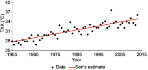
We modeled the data series through the GEV distribution of three parameters, using stationary and non-stationary models for periods that varied from 83 years (Veracruz) to 31 years (Tuxtla Gutiérrez); the other cities had intermediate periods (Table I). The inclusion of non-stationarity is plausible for our modeling approach, as can be visualized for many locations. As an example, time series of TXX (Figs. 4, 6, 8, and 10) and TNN (Figs. 5, 7, 9, and 11) are shown for four of the 12 urban areas (Tijuana, Guadalajara, Toluca, and Puebla), with a trend line using Sen’s slope estimator. The graphs for several cities show a clear trend in the maximum and minimum annual data. The graphical analysis and results of the Mann-Kendall trend test justify the use of non-stationary GEV models over time as a covariate. The trends shown are statistically significant with a p-value < 0.05, except for the TXX of Toluca, whose trend is significant with a p-value < 0.1, and the TXX of Tijuana, whose trend is not significant.


The time series of TXX and TNN were used to estimate the parameters in the distribution of GEV with and without trends, as well as the periods of return. The models were adjusted to the maximum annual temperature and minimum annual temperature of each of the 16 climate stations using the maximum likelihood (ML) method.
An attempt was made to improve the modeling approach by allowing the location parameter (μ) to depend on time. As mentioned, three model selection criteria (AIC, BIC, and LRT) were used to select the best model from a collection of nested models. The best adjustment models for TXX and TNN through the GEV distributions, as selected by the criteria separately listed for each urban area, are summarized in Table II.
Table II Parameter estimates and criteria of the constant and linear models for µ in the generalized extreme values (GEV) model applied to temperature extreme data.
| City | GEV parameters | TXX | TNN |
| Aguascalientes | Constant model: µ, σ, ξ, AIC, BIC Linear model: µ 0 , µ 1 , σ, ξ, AIC, BIC, LRT | 34.25, 1.37, -0.066, 251.19, 257.76 33.9, 0.009, 1.33, -0.028, 252.31, 261.07, 0.88 | -2.29, 2.26, -0.35, 296.46, 303.03 -4.4, 0.073, 1.90, -0.57, 259.54, 268.3, 38.9* |
| Mexicali | Constant model: µ, σ, ξ, AIC, BIC Linear model: µ 0 , µ 1 , σ, ξ, AIC, BIC, LRT | 46.74, 1.38, -0.17, 231.76, 238.19 45.87, 0.03, 1.31, -0.18, 226.39, 234.91, 7.36* | -1.73, 2.91, -0.49, 305.21, 311.6 -4.13, 0.08, 2.28, -0.49, 275.81, 284.38, 31.4* |
| Tijuana | Constant model: µ, σ, ξ, AIC, BIC Linear model: µ 0 , µ 1 , σ, ξ, AIC, BIC, LRT | 38.03, 2.17, -0.23, 285.58, 292.01 37.14, 0.03, 2.10, -0.24, 283.71, 292.29, 3.87* | 1.14, 1.06, 0.04, 215.85, 222.28 027, 0.03, 1.05, -0.14, 202.9, 211.48, 14.95* |
| Tuxtla Gutiérrez | Constant model: µ, σ, ξ, AIC, BIC Linear model: µ 0 , µ 1 , σ, ξ, AIC, BIC, LRT | 40.29, 1.27, -0.70, 94.30, 98.61 40.33, -0.003. 1.25, 96.13, 101.86, 0.18 | 10.48, 1.46, -0.45, 111.66, 115.96 9.06, 0.09, 1.17, -0.47, 99.10, 104.84, 14.55* |
| Úrsula Coapa (CDMX) | Constant model: µ, σ, ξ, AIC, BIC Linear model: µ 0 , µ 1 , σ, ξ, AIC, BIC, LRT | 32.22, 1.58, -0.36, 162.98, 168.27 31.53, 0.03, 1.46, -0.27, 163.25, 170.3, 1.73 | 0.57, 1.55, -0.15, 171.35, 176.63 -0.71, 0.061, 1.32, -0.10, 161.25, 168.3, 12.1* |
| Gran Canal (CDMX) | Constant model: µ, σ, ξ, AIC, BIC Linear model: µ 0 , µ 1 , σ, ξ, AIC, BIC, LRT | 32.1, 1.23, -0.04, 206.15, 212.28 32.32, -0.008, 1.21, -0.032, 207.33, 215.5, 0.81 | |
| Milpa Alta (CDMX) | Constant model: µ, σ, ξ, AIC, BIC Linear model: µ 0 , µ 1 , σ, ξ, AIC, BIC, LRT | 28.59, 1.49, -0.15, 167.85, 173.13 29.19, -0.03, 1.38, -0.08, 167.29, 174.33, 2.56 | -0.50, 1.66, -0.43, 163.89, 169.17 0.22, -0.04, 1.48, -0.26, 164.35, 171.39, 1.54 |
| León | Constant model: µ, σ, ξ, AIC, BIC Linear model: µ 0 , µ 1 , σ, ξ, AIC, BIC, LRT | 35.03, 1.39, -0.19, 207.23, 213.31 34.53, 0.02, 1.35, -0.17, 207.23, 213.21, 2.1 | 1.47, 1.83, -0.34, 228.35, 234.42 -0.46, 0.08, 1.58, -0.56, 198.74, 206.84, 31.6* |
| Guadalajara | Constant model: µ, σ, ξ, AIC, BIC Linear model: µ 0 , µ 1 , σ, ξ, AIC, BIC, LRT | 35.48, 1.27, -0.24, 197.58, 203.71 36.61, -0.04, 1.16, -0.28, 186.47, 194.64, 13.1* | 4.35, 2.62, -0.53, 261.87, 268.0 1.61, 0.10, 2.19, -0.61, 238.0, 246.17, 25.9* |
| Aculco (ZMVM) | Constant model: µ, σ, ξ, AIC, BIC Linear model: µ 0 , µ 1 , σ, ξ, AIC, BIC, LRT | -2.15, 2.09, -0.61, 171.99, 177.2 0.93, -0.13, 1.66, -0.79, 145.48, 152.43, 28.5* | |
| Toluca (ZMVM) | Constant model: µ, σ, ξ, AIC, BIC Linear model: µ 0 , µ 1 , σ, ξ, AIC, BIC, LRT | 27.71, 1.39, -0.04, 141.63, 146.38 26.61, 0.06, 1.18, 0.047, 136.14, 142.47, 7.5* | -7.1, 1.46, -0.25, 136.5, 141.25 -8.4, 0.08, 1.27, -0.34, 126.02, 132.35, 12.5* |
| Chapingo (ZMVM) | Constant model: µ, σ, ξ, AIC, BIC Linear model: µ 0 , µ 1 , σ, ξ, AIC, BIC, LRT | 32.18, 1.39, -0.15, 213.29, 219.42 30.87, 0.05, 1.17, -0.17, 194.2, 202.37, 21.1* | -3.73, 2.07, -0.35, 245.61, 251.74 -5.65, 0.07, 1.75, -0.39, 226.11, 234.28, 21.5* |
| Monterrey | Constant model: µ, σ, ξ, AIC, BIC Linear model: µ 0 , µ 1 , σ, ξ, AIC, BIC, LRT | 40.19, 1.91, -0.16, 263.31, 269.65 40.49, -0.01, 1.89, -0.16, 264.84, 273.29, 0.47 | -1.25, 3.39, -0.51, 311.1, 317.42 -2.64, 0.06, 3.84, -0.73, 299.38, 307.83, 13.7* |
| Puebla | Constant model: µ, σ, ξ, AIC, BIC Linear model: µ 0 , µ 1 , σ, ξ, AIC, BIC, LRT | 30.25, 2.37, -0.25, 277.3, 283.53 27.1, 0.12, 0.99, -0.07, 187.62, 195.92, 91.7* | -0.46, 1.46, -0.24, 220.31, 226.55 -1.96, 0.05, 1.15, -0.15, 200.58, 208.89, 21.7* |
| Tlaxcala | Constant model: µ, σ, ξ, AIC, BIC Linear model: µ 0 , µ 1 , σ, ξ, AIC, BIC, LRT | 31.64, 1.19, 0.11, 169.51, 174.93 31.53, 0.005, 1.19, 0.10, 171.3, 178.5, 0.21 | -2.51, 1.63, -0.49, 166.1, 171.5 -3.53, 0.05, 1.5, -0.66, 153.47, 160.7, 14.6* |
| Veracruz | Constant model: µ, σ, ξ, AIC, BIC Linear model: µ 0 , µ 1 , σ, ξ, AIC, BIC, LRT | 34.5, 1.46, 0.10, 349.1, 356.4 33.01, 0.04, 1.12, 0.14, 310.55, 320.32, 40.5* | 12.41, 1.73, -0.44, 323.97, 331.3 12.32, 0.002, 1.73, -0.44, 325.8, 335.57, 0.17 |
TXX: extreme maximum temperature; TNN: extreme minimum temperature; CDMX: Mexico City; ZMVM: metropolitan area of the Valley of Mexico; AIC: Akaike information criteria; BIC: Bayes information criteria; LRT: likelihood ratio test.
μ0, μ1, σ, ξ are parameters of the GEV distribution defined in Eqs. (1) and (2).
*Significance at the 95% confidence level.
In total, 58 models were generated. Table II shows the resulting estimators and the criteria for selecting the best model to be used in the estimation of return periods. According to this table, for the temporal trend of TXX, significant at a 95% confidence level, it can be seen that: (a) 44% of locations (seven urban areas) show a significant trend, (b) 50% of locations (eight urban areas) have no significant trend, and (c) 6% of locations (one urban area) show no trend. For the temporal trend of TNN, also significant at the 95% confidence level, it was found that: (a) 82% of locations (13 urban areas) show a significant trend, (b) 12% of locations (two urban areas) show no significant trend, and (c) 6% of locations (one urban area) show no trend.
According to the shape parameter (ξ), and by performing a detailed analysis, it was found that for the case of TXX, 63% of the climatic stations were adjusted to the Weibull distribution (ξ < 0), 25% were adjusted to the Gumbel distribution, 6% were adjusted to the Fréchet distribution, and 6% did not fit any of the three distributions. In the case of TNN, 94% of the analyzed climatic stations were adjusted to the Weibull distribution, and only 6% did not adjust to any of the distributions.
In the case of TXX, which exhibits a significant temporal trend, it was found that 72% was adjusted to the Weibull distribution, 14% to the Gumbel distribution, and 14% to the Fréchet distribution. For TNN, it was found that those that show a significant temporal trend (82%) and those that are stationary (12%) conformed to the Weibull distribution.
Overall, for both extreme temperatures TXX and TNN, it was found that the 57% following the Weibull distribution are statistically significant to the temporal trend at the 95% confidence level. One of the properties of this distribution, which may even be controversial because of the trend found, is that both extreme temperatures have an upper limit that cannot be exceeded.
Figures 12 and 13 describe the temporal trend pattern of decadal trends for the location parameter (μ) of the maximum and minimum temperatures according to non-stationary GEV models (Table II). About the TXX (Fig. 12), the most significant positive trend occurred in the center and east regions (Toluca, Chapingo, Puebla and Veracruz), whereas the lowest trends occurred in the northwest regions (Tijuana and Mexicali).
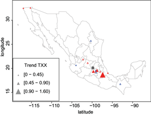
Fig. 12 Spatial patterns of trends of the location parameter (μ) for the maximum temperature. Red (blue) triangles mean positive (negative) values. Full triangles mean significant trends at the 5% level. The symbol ⊗ indicates without change.
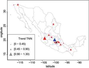
Fig. 13 Spatial patterns of trends of the location parameter (μ) for the minimum temperature. Red (blue) triangles mean positive (negative) values. Full triangles mean significant trends at the 5% level.
Respect to the TNN (Fig. 13), the most significant positive trends were most relevant in different geographical areas of the country, i.e., higher in the west center (Guadalajara and León), southeast (Tuxtla Gutiérrez), some urban areas located in the central part (Úrsula Coapa, Toluca, Chapingo, Tlaxcala and Puebla), and in the northeast and northwest (Monterrey and Mexicali), whereas the lowest positive trend occurred in the urban area of Tijuana (with a value of 0.30). The most significant negative trend occurred in an urban area.
Once the best models were selected, the return levels of the extreme, maximum, and minimum temperatures were estimated. Tables III and IV present the estimators and confidence intervals for return levels to 10, 20, 50, and 100 years, for both stationary and non-stationary models. The stationary return levels for TXX in Table III, indicate that the values increase for increasingly larger periods (10, 20, 50, and 100 years), except for the urban area of Tuxtla Gutiérrez. In addition, the confidence intervals were increasingly wider as the periods of return increased. In Aguascalientes the TXX can be expected to progressively exceed 37.1 ºC on average every 10 years, 37.9 ºC on average every 20 years, 38.9 ºC on average every 50 years, and 39.7 ºC on average every 100 years. The 95% confidence intervals for these return periods, in ºC, were 36.4-37.8, 37.0-38.9, 37.5-40.4, and 37.8-41.5, respectively.
Table III Stationary and non-stationary return levels for extreme maximum temperature and its 95% confidence levels (in parentheses).
| Urban zone | Return levels (10 years) | Return levels (20 years) | Return levels (50 years) | Return levels (100 years) |
| Stationary return levels (ºC) | ||||
| Aguascalientes | 37.1 (36.4-37.8) | 37.9 (37.0-38.9) | 38.9 (37.5-40.4) | 39.7 (37.8-41.5) |
| Tuxtla Gutiérrez | 41.7 (41.5-42.0) | 41.9 (41.7-42.0) | 42.0 (41.8-42.2) | 42.0 (41.8-42.2) |
| Úrsula Coapa | 34.7 (34.2-35.2) | 35.1 (34.6-35.6) | 35.5 (35.0-36.1) | 35.8 (35.1-36.4) |
| Gran Canal | 34.7 (34.0-35.4) | 35.5 (34.6-36.5) | 36.5 (35.1-37.9) | 37.2 (35.4-39.1) |
| Milpa Alta | 31.4 (30.7-32.2) | 32.2 (31.2-33.1) | 33.0 (31.8-34.2) | 33.6 (32.0-35.1) |
| León | 37.6 (37.0-38.1) | 38.2 (37.5-38.9) | 38.9 (37.9-39.8) | 39.3 (38.8-40.4) |
| Monterrey | 43.8 (43.0-44.6) | 44.7 (43.8-45.6) | 45.7 (44.6-46.9) | 46.4 (45.0-47.7) |
| Tlaxcala | 34.7 (33.6-35.8) | 35.8 (34.1-37.6) | 37.5 (34.4-40.5) | 38.8 (34.5-43.2) |
| Non-stationary return levels (ºC) | ||||
| Mexicali | 48.5 (48.0-49.1) | 49.4 (48.8-50.1) | 50.9 (50.1-51.7) | 52.7 (51.7-53.7) |
| Tijuana | 41.1 (40.3-41.8) | 42.2 (41.3-43.0) | 43.9 (42.8-45.0) | 45.9 (44.5-47.2) |
| Guadalajara | 38.2 (37.8-38.7) | 38.3 (37.7-38.8) | 37.6 (36.9-38.3) | 36.1 (35.2-36.9) |
| Toluca | 30.0 (28.9 -31.0) | 31.5 (30.1-32.9) | 34.6 (32.4-36.8) | 38.6 (35.7-41.5) |
| Chapingo | 33.5 (32.9-34.1) | 34.5 (33.8-35.3) | 36.6 (35.6-37.6) | 39.5 (38.2-40.7) |
| Puebla | 30.2 (29.4-31.0) | 32.0 (31.0-32.9) | 36.3 (35.1-37.5) | 42.8 (41.4-44.2) |
| Veracruz | 36.3 (35.3-37.3) | 37.9 (36.2-39.5) | 40.7 (37.9-43.5) | 44.0 (40.0-48.1) |
Among the locations considered in that block, and in the context of the stationary return levels, Monterrey (in the northeast of the country) was associated with the highest return levels, and Milpa Alta (in the metropolitan area of the Valley of Mexico in the center of the country) had the lowest return levels. Based on the 95% confidence interval and according to Table III, we can expect that the largest TXX event recorded for Milpa Alta could reappear for the next 10 years. Moreover, there is a high probability that the annual TXX will exceed the maximum historical value in the next 50 years, except in the sites Gran Canal and Monterrey.
The estimated return levels assume stationarity, meaning that the level of return for a return period is the same for the successive years. This implies that the statistical properties of the parameters μ, σ, and ξ are constant.
In a non-stationary case, the parameters of the GEV distribution vary over time, and the return levels of extreme temperatures will also follow that temporal trend. Under a changing climate, the return value can be interpreted as an extreme quantile of a temperature distribution that varies over time (for example, a return value of 20 years can be interpreted as a value that has a 5% probability to be exceeded in a particular year).
It is now possible to estimate return levels for any year, which are also presented in Table III. For example, note that the average return levels (in ºC) for Mexicali for 10, 20, 50, and 100 years, are 48.5, 49.4, 50.9 and 52.7, respectively. The confidence intervals at 95% (in º C) are 48.0-49.1, 48.8-50.1, 50.1-51.7, and 51.7-53.7, respectively. The differences in return levels between stations is remarkable, both in the stationary GEV models and in the non-stationary models. Mexicali, in the northwest of Mexico, is associated with the highest return levels, whereas Milpa Alta, a metropolitan area in Mexico City, has the lowest return levels.
With respect to TNN, Table IV shows that only stations Milpa Alta and Veracruz have stationary return levels, and that the values increase slightly for increasingly large return periods (10, 20, 50, and 100 years). In addition, the confidence intervals remain nearly constant as the periods of return increase. For example, Milpa Alta could expect the TNN to exceed 1.9 ºC on average every 10 years, 2.3 ºC on average every 20 years, 2.6 ºC on average every 50 years, and 2.8 ºC on average every 100 years. The confidence intervals, at 95% (in ºC) are 1.4-2.3, 1.8-2.7, 2.2-3.1, and 2.3-3.3, respectively.
Table IV Stationary and non-stationary return levels for extreme minimum temperature and its 95% confidence levels (in parentheses).
| Urban zone | Return levels (10 years) | Return levels (20 years) | Return levels (50 years) | Return levels (100 years) |
| Stationary return levels (ºC) | ||||
| Milpa Alta | 1.9 (1.4-2.3) | 2.3 (1.8-2.7) | 2.6 (2.2-3.1) | 2.8 (2.3-3.3) |
| Veracruz | 14.9 (14.6-15.2) | 15.3 (15.0-15.6) | 15.6 (15.3-16.0) | 15.8 (15.5-16.2) |
| Non-stationary return levels (ºC) | ||||
| Aguascalientes | -1.3 [-1.9-(-0.7)] | -0.3 [-1.0-(0.4)] | 2.1 (1.3-3.0) | 5.9 (4.9-7.0) |
| Mexicali | -0.3 [-0.9-(0.3)] | 1.0 (0.4-1.6) | 3.8 (3.1-4.5) | 8.0 (7.1-8.8) |
| Tijuana | 2.6 (1.8-3.4) | 3.4 (2.2-4.7) | 5.0 (2.8-7.3) | 7.1 (3.9-10.3) |
| Tuxtla Gutiérrez | 11.5 (11.1-12.0) | 12.7 (12.3-13.2) | 15.8 (15.2-16.3) | 20.6 (19.9-21.2) |
| Úrsula Coapa | 2.5 (1.7-3.3) | 3.8 (2.9-4.8) | 6.5 (5.3-7.8) | 10.2 (8.6-11.8) |
| León | 2.3 (1.7-2.8) | 3.3 (2.7-3.8) | 5.8 (5.2-6.5) | 9.8 (9.0-10.5) |
| Guadalajara | 5.2 (4.7-5.7) | 6.5 (6.1-7.0) | 9.8 (9.3-10.2) | 14.9 (14.4-15.4) |
| Aculco | 2.6 (2.2-2.9) | 2.6 (2.3-2.9) | 2.3 (1.9-2.7) | 1.7 (1.3-2.1) |
| Toluca | -5.7 [-6.4-(-5.0)] | -4.6 [-5.3-(-3.8)] | -1.9 [-2.9-(-0.8)] | 2.2 (1.0-3.4) |
| Chapingo | -2.4 [-3.0-(-1.8)] | -1.2 [-1.8-(-0.6)] | 1.3 (0.6-2.0) | 5.1 (4.3-5.9) |
| Monterrey | 2.1 (1.5-2.8) | 3.1 (2.5-3.7) | 5.1 (4.5-5.6) | 8.0 (7.5-8.6) |
| Puebla | 0.7 (0.2-1.2) | 1.8 (1.2-2.4) | 3.9 (3.2-4.7) | 6.9 (6.0-7.8) |
| Tlaxcala | -1.3 [-1.7-(-1.0)] | -0.6 [-1.0-(-0.3)] | 1.0 (0.6-1.3) | 3.5 (3.1-3.9) |
As already mentioned, the estimated return levels assume stationarity, meaning that the level of return for a return period is the same for successive years. This also implies that the statistical properties, as mentioned for TXX, keep the parameters μ, σ, y, and ξ constant.
In a non-stationary case (as with TXX), the parameters vary in time and the return levels of extreme temperatures will follow a similar temporal trend. It is possible to estimate return levels for any year of interest in a time period. The return levels for the non-stationary TNN series are presented in Table IV. Note that the average return levels of 10, 20, 50, and 100 years (in ºC) for Aguascalientes are -1.3, -0.3, 2.1, and 5.9, respectively, whereas their confidence intervals, at 95% and in ºC, progress from -1.9 to -0.7, -1.0 to 0.4, 1.3 to 3.0, and 4.9 to 7.0, respectively.
In the case of a non-stationary series, for both TXX and TNN, a positive trend of the location parameter (μ 1 ) will be reflected in the positive trend of the return levels (Chen and Chu, 2014). This means that with greater magnitudes of the trend return levels will increase considerably, and threshold values of return levels will contain greater variation over time. As examples of estimators of return levels, the time series of return levels for TXX for the city of Puebla (Fig. 14) and for TNN for the city of Guadalajara (Fig. 15) are plotted, according to the GEV adjustment non-stationary model. The difference in the return level for 2 years for the city of Puebla from the beginning of the period (1955) to the end (2013) is approximately 5 ºC, whereas the difference in the return level of 2 years for the city of Guadalajara from the beginning of the period (1957) to the end (2013) is approximately 3 ºC.
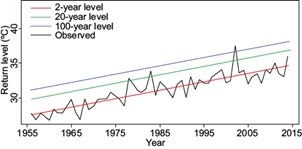
Fig. 14 Time series of extreme maximum temperature (TXX) return levels in Puebla in accordance with the non-stationary generalized extreme value (GEV) model. The red, green, and blue lines represent the return levels of 2, 20, and 100 years, respectively. The black line represents observed values.
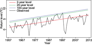
Fig. 15 Time series of extreme minimum temperature (TNN) return levels in Guadalajara in accordance with the non-stationary GEV model. The red, green, and blue lines represent the return levels of 2, 20, and 100 years, respectively. The black line represents observed values.
The application of the stationary and non-stationary GEV distributions has allowed this study to model the behavior of extreme temperatures in some cities of Mexico. Due to the lack of reliable data, only 16 climate stations were used, focusing on 12 urban areas. The latitudinal dispersion of these climatic stations ranged from 16º 45’ (Tuxtla Gutiérrez) to 32º 39’ (Mexicali), and with altitudes above sea level varying from 4 m (Mexicali) to 2726 m (Toluca). This resulted in several types of climates according to the geographical location (García-Cueto et al. 2018), making the analysis by chosen city even more interesting. This is particularly true for those cities that show significant trends and periods of return that could put the adaptation of people and the urban ecosystem at risk, particularly the fauna and flora. We found that the TXX is increasing in Mexicali, Tijuana, Toluca, Chapingo, Puebla and Veracruz, and no significant changes were detected in the other 10 urban zones. A larger number of climatological stations indicate increasing TNN compared to TXX, namely Aguascalientes, Mexicali, Tijuana, Tuxtla Gutiérrez, Úrsula Coapa, León, Guadalajara, Aculco, Toluca, Chapingo, Monterrey, Puebla and Tlaxcala. Non significant increases were detected in only two stations, i.e., Milpa Alta and Veracruz.
A comparison of the obtained results with those from studies using the ETCDDI indices shows similarities and some differences. For example, García-Cueto et al. (2018) used the same database herein and found a statistically significant increasing trend in the TX90 (warm days) and TN90 (warm nights) indices for Aguascalientes, whereas for Milpa Alta, both indices (TX90 and TN90) decreased significantly. The difference is between the TXX (stationary in this study) and TX90 (increasing trend) for Aguascalientes; in the case of Milpa Alta, there are coincidences in both indices (TXX with TX90 and TNN with TN90) that show decreasing trends.
At the country level, according to Gosling et al. (2011), Mexico has experienced a generalized warming since 1960. The frequency of cold days has decreased, and the frequency of warm nights has increased. There has also been a general increase in average winter temperatures in the country as a result of human influences on climate. Thus, during the winter season, the occurrences of warm temperatures are more frequent, and those of cold temperatures are less frequent. For the A1B emissions scenario, the projected temperature increases of the Coupled Model Intercomparison Project Phase 3 (CMIP3) over Mexico are approximately 4 ºC near the US border, with increases in the rest of the country between 2.5 and 3.5 ºC. This implies that the influence of GHGs will have an additive effect on the potential warming caused by urbanization. This can become a major problem affecting city dwellers both positively and negatively, depending on their latitudinal location.
Significant trends in extreme maximum and minimum temperatures found in many parts of the world (Heim Jr., 2015; Easterling et al., 2016; Houngninou et al., 2017) reinforce the results obtained here. In the US, extremely hot maximum and minimum temperatures have shown increasing trends between the 20th and 21st centuries and during the last four decades (1971-2013), whereas the presence of extremely low and minimum temperatures has decreased during these periods (Hartmann et al., 2013).
The application of a theory of extreme events to the TXX and TNN in 16 climatological stations located in 12 urban areas of Mexico, in time series with different periods, showed general trends in urban warming, especially at night. However, values varied from city to city. A less clear detection signal was the diurnal heating. Although the causes for this behavior of heterogeneous trends for TXX and TNN may be of purely local origin and caused by the dynamics of urbanization (land use change, anthropogenic activities), it cannot be ruled that they could be caused by some other climatic phenomena of a greater scale. For example, Mexico could be exposed to blocking patterns, or modes of climate variability, such as the El Niño Southern Oscillation, Pacific Decadal Oscillation, North Atlantic Oscillation, or the Madden-Julian Oscillation, among others. These could be causal factors that contribute to thermal trends since in other regions of the world they have significantly influenced the behavior of extreme temperatures (Arblaster and Alexander, 2012; Parker et al., 2014; Burgess and Klingaman, 2015; Matsueda and Takaya, 2015). All these factors are considered important for possible attribution but are not the object of this study.
It is well known that cities will remain the most vulnerable geographic spaces, especially in developing countries such as Mexico, as they often concentrate large populations without adequate infrastructure. Thus, knowledge of regions where the climate is unstable (changing), and the knowledge that extreme climate events are not controllable, but have showed signals of an increasing trend, will serve to generate some potential urban adaptation strategies for facing current and future extreme temperatures. For example, such temperatures can be addressed by redesigning the urban space (making it safe, ecological and acceptable) to reduce vulnerability and strengthen urban water security. It should be noted that each city is a case of analysis, and that an adequate scheme of sustainable urban planning can only be accomplished through the participation of governmental authorities, productive sectors, academics, and local actors.
6. Conclusions
This study modeled the TXX and TNN recorded in 16 climatological stations corresponding to 12 cities in Mexico, for periods that varied according to the series of available data. The longest record corresponded to Veracruz with 85 years (1930-2014), and the shortest to Tuxtla Gutiérrez with 31 years (1980-2010). Through the application of the non-parametric Mann-Kendall test and the Sen method, a trend towards urban warming was detected, but no homogeneous behavior in all cities analyzed was found. An important observation was the significant prevalence of non-stationary series with the TXX in half of the cities analyzed; only Guadalajara, located in the center-west of the country, presented a significant negative trend, perhaps due the effect of “diming” by increases in aerosol pollution (Fonseca-Hernández et al., 2018). Therefore, the annual trends in daytime warming, represented by TXX, are not necessarily identical in all selected urban areas of Mexico. In the case of the TNN, which is related to night warming, the behavior was more uniform. Specifically, 90% of the cities are non-stationary with a significant positive trend, and only two areas presented a stationary series: one urban area located to the east of the metropolitan area of the Valley of Mexico (Milpa Alta), and another on the coast of the Gulf of Mexico (Veracruz). With the adjustment of the non-stationary GEV distribution to the data set and by incorporating the trend of the location parameter, the trends of the return levels of 10, 20, 50, and 100 years were estimated, while keeping the shape and scale parameters constant.
The results are very similar to those from non-parametric trend detection methods, both for TXX and TNN. This confirms the non-stationary behavior of half of the stations for TXX, and 90% of the stations for TNN. Return periods of the thermal extremes estimated in a changing climate for many of the cities analyzed in this study vary significantly, and the regularity with which extreme temperatures are occurring is becoming more frequent. Thus, statistical modeling should consider this behavior, due to its importance for risk assessments for human health, flora and fauna, and urban infrastructure. The proposed non-stationary GEV model has provided new and important information concerning changes in extreme temperatures, and by estimating return periods, it has provided their probability of recurrence. Some main modes of climate variability as causal mechanisms of attribution of extreme temperatures have not been studied, making it a pending task.

