


 nueva página del texto (beta)
 Inglés (pdf)
 Artículo en XML
 Referencias del artículo
 Enviar artículo por email
 Citado por SciELO
  Similares en
SciELO
Similares en
SciELO 
 Permalink
1. Introduction
Carbon monoxide (CO) is a gas emitted mainly at the surface level by fossil fuels combustion and biomass burning (Kerzenmacher et al., 2012, Stremme et al., 2013). In the atmosphere it is produced and removed by hydrocarbons oxidation and chemical reaction with the hydroxyl radical (OH), respectively. Due to its lifetime of weeks to a few months in the troposphere, depending on where it is analyzed and the season of the year, CO has been used as an atmospheric transport tracer (Rinsland et al., 2006; de Foy et al., 2007; Funke et al., 2007; Turquety et al., 2008, 2009; George et al., 2009; de Wachter et al., 2012).
CO is not only measured in surface but also at different altitudes employing remote sensing, such as satellite measurements from the Measurement of Pollution in the Troposphere (MOPITT), the Scanning Imaging Absorption Spectrometer for Atmospheric Chartography (SCIAMACHY), and the Infrared Atmospheric Sounding Interferometer (IASI), among other instruments (Luo et al., 2007; Clerbaux et al., 2008a; Turquety et al., 2008). These observations can also provide information of CO surface concentrations and its transport over polluted urban areas (Clerbaux et al., 2008b; Fortems-Cheiney et al., 2009; Fagbeja et al., 2015; Rakitin et al., 2015; Bauduin et al., 2016).
Several studies have been carried out around the world employing satellite observations, e.g., Liu et al. (2005) studied the MOPPIT detection of CO emission from large forest fires in the United States during 2000; Tanimoto et al. (2009) analyzed CO plumes transported from western Siberia toward northern Japan using images from the Atmospheric Infrared Sounder (AIRS); Kopacz et al. (2009) constrained Asian sources of CO by using an atmospheric chemical transport model (GEOS-Chem CTM) and observations from MOPITT; Klonecki et al. (2012) evaluated the IASI CO product against independent in-situ aircraft and analyzed the impact of eight months assimilation of IASI CO columns; Marey et al. (2015) presented a satellite-based analysis to explore contributing factors that affect tropospheric CO levels over Alberta, Canada, and Rakitin et al. (2017) estimated trends of total CO over Eurasia using information from AIRS.
Previous studies have been carried out in Mexico City and its surrounding metropolitan area, such as the conducted by de Foy et al. (2007), in which vertical column measurements of CO, derived from Fourier Transform Infrared (FTIR) spectrometers, were used to constrain the CO emission in models, and the CO emission was also evaluated in the inventory for this region; Stremme et al. (2013) presented a new methodology for estimating CO emissions on large urban areas based on a top-down approach using FTIR measurements from ground and space (employing the IASI instrument), and Bauduin et al. (2016) investigated the capability of IASI to retrieve near-surface CO concentrations and evaluated the influence of thermal contrast. These works focused on analyzing CO emissions in Mexico City, but it is important to study other surrounding regions.
Regarding IASI, it is one of the most recent satellite instruments that measure CO. It was launched in 2006 on board the Metop-A satellite. The field of view is 50 km with four circular measurements of 12 km at nadir and has a swath of 2200 km that allows to observe the planet twice a day (Clerbaux et al., 2009; Hilton et al., 2012). The satellite is sun-synchronous with equator crossing times of 09:30 and 21:30 LT (Clerbaux et al., 2009; Fortems-Cheiney et al., 2009; George et al., 2009; Turquety et al., 2009) and the crossing hour over central Mexico is approximately at 10:00 LT (Stremme et al., 2013). In addition, IASI has a resolution of 0.5 cm-1 in a spectral range from 645 to 2760 cm-1.
This work aims to reduce the differences between the observed and modeled carbon monoxide concentrations by employing the WRF-Chem model fed with the 2008 emissions inventory. To do this, a methodology was applied to compare WRF-Chem and IASI data, obtaining scaling factors that allow to update carbon monoxide emissions for a specific period.
2. Methodology
2.1 Model and data description
The WRF-Chem model (Grell et al., 2005; Fast et al., 2006) was used to estimate CO concentrations. The model was fed with NCAR one-degree resolution meteorological data and two nested domains were modeled using the USGS 24-category land-use: the first one with a 90 by 90 cells mesh grid with 9-km resolution and the second with an 88 by 88 cells mesh grid with 3-km resolution (Fig. 1). February 2011 was modeled because it was the month with more available surface measurement data (from a campaign carried out in the State of Mexico). The parameterizations employed in this work are the YSU scheme for the boundary layer (Song-You et al., 2006), the WRF Single-Moment 5-class scheme (WSM5) for microphysics (Song-You et al., 2004), Rapid Radiative Transfer Model scheme (RRTM) for the longwave radiation (Mlawer et al., 1997), the Goddard scheme for the shortwave radiation (Matsui et al., 2018) and the Grell-3 scheme for the cumulus option (Grell, 1993; Grell et al., 2002)

Fig. 1 Modeling domains (white squares). The largest domain has a 9-km resolution and the smallest a 3-km resolution.
The 2008 National Emissions Inventory (García- Reynoso et al., 2018) was used because at the time of the analysis only these emission data were available. The National Emissions Inventory was developed by the Mexican Ministry of Environment and Natural Resources (SEMARNAT). It includes information on emissions released into the atmosphere from criteria pollutants: carbon monoxide (CO), nitrogen oxides (NOx), sulfur oxides (SOx) and particles with aerodynamic diameter less than 10 and 2.5 µm (PM10 and PM2.5), volatile organic compounds (VOCs) and ammonium (NH3), emitted from area, mobile and fixed sources. It is elaborated periodically and is available from the internet (https://www.gob.mx/semarnat/documentos/documentos-del-inventario-nacional-de-emisiones). Its elaboration follows international standards, and it has some quality assurance procedures for the input, the processing and the reporting of information. The annual emissions inventory was processed in order to be suitable to use in the WRF-Chem model following the methodology presented by García-Reynoso et al. (2018).
Regarding the satellite data, we used the Fast Optimal Retrievals on Layers for IASI (FORLI-CO) (https://iasi.aeris-data.fr/CO_IASI_A_data/), which calculates the CO profile in 19 layers with a 1-km thickness in the first 18 layers and up to a 60-km altitude in the last one (Hurtmans et al., 2012; de Wachter et al., 2012). All the CO total column data were obtained at 10:00 LT, approximately (Stremme et al., 2013), including the averaging kernel matrix, its associated errors, and the a priori profile, among other values.
In order to compare the model results against surface observations, data from five stations of Mexico City’s Automatic Air Quality Monitoring Network (RAMA, Spanish acronym) were used: Iztacalco (IZT), Merced (MER), Santa Úrsula (SUR), Tlalnepantla (TLA) and UAM Iztapalapa (UIZ). This monitoring network reports hourly concentrations of CO, SO2, O2, and NOx, among other chemical and meteorological variables. In addition, the United States Environmental Protection Agency (USEPA) has been performing audits to stations within Mexico City’s air monitoring network since 2009, evaluating their systems for station operation and calibration (http://www.aire.cdmx.gob.mx/default.php?opc=%27ZaBhnmI=&dc=%27Zg==).
Additionally, data from a surface measurement campaign in the State of Mexico were used in the Amecameca (AME), Tenango (TEN) and Ozumba (OZU) municipalities (Fig. 2).

2.2 Modeling procedure
Dedicated CO emission inventories were created for the 3-km resolution model domain. These inventories only have CO emissions for some specific regions: The Mexico City Metropolitan Area (MCMA), the Toluca and Lerma municipalities, and Morelos, Puebla and Hidalgo states (Fig. 3). A zero-emission value was placed on the remaining domain areas and the concentration from model boundaries was considered.

Fig. 3 Metropolitan areas that were used to evaluate the influence of surrounding cities over the MCMA.
Subsequently, the WRF-Chem model was run for February 1-28, 2011. The chemistry was turned off in order to model five tracers (considering the concentration from model boundaries) with the purpose of knowing the influence of each region on the others.
2.2.1 Model total column calculation procedure
It is known that the satellite crossing time over central Mexico is around 10:00 LT (Clerbaux et al., 2009; Stremme et al., 2013). Therefore, the comparisons between satellite and modeled data are made at this time. For this, it is necessary to compute the CO modeled columns (in molecules per cm2) for each grid by using the concentration in every level (in parts per million in volume [ppm]), temperature, pressure and layer thickness (Lt).
First, the model height of each level and the thickness of each layer are obtained:
where L t is the layer thickness (m), Z the level height in meters (m), PH the geopotential height (m2s-2), and PHB the geopotential perturbation (m2s-2).
Then, the state equation is used for the calculation of molecules cm-2:
where
C co is the CO concentration in ppm (mL m-3), R = 82.57 (mL atm mol-1 K-1), NA is the Avogadro number (molecules mol-1), P model is the model pressure (Pa), PB is the pressure perturbation (Pa), and T:
where Tmodel is the perturbation potential temperature (θ - T 0 ) (K), (T 0 = 300), and P 0 the reference pressure (1 atm).
Then, this method allows to estimate the modeled partial columns for each layer in the model.
2.2.2 Scaling factors calculation procedure
According to Rodgers and Connor (2003), in order to compare total columns from different instruments that have different characteristics and vertical sensitivity, it is necessary to perform a data treatment that includes some of their characteristics. In this case, IASI’s averaging kernels were used, which provide information about the vertical sensitivity of the retrieval to the true state of the atmosphere (Eq. [6a]) (Rodgers, 2000; Luo et al., 2007).
where x sat is the retrieved profile, x a the IASI a priori profile, Asat the IASI’s averaging kernels, x true the true but unknown profile, and ε the error in the retrieved profile.
For the comparison, we assume that the modeled profile is the true profile.
Therefore, the satellite averaging kernels were first interpolated to the model heights in each coincident point. Next, the modeled CO profiles were smoothed by using Eq. (6b):
where x model_smoothed is the smoothed model profile, A the averaging kernel interpolated to model heights, and x model the original model profile.
In this work we used the satellite total column. Then, the total column operator was applied for modeled partial columns (g = [111111….1]) to sum up all modeled partial columns:
Afterwards, a matrix K was created. Its columns correspond to the smoothed total column values calculated by Eq. (6c) for each region and the concentration from model boundaries. Its rows indicate the number of coincident points between the satellite and the model. Therefore, in this specific work: K (1074,6).
The modeled CO total column of each grid point and time is a linear combination of different origin CO molecules sum, which is represented by Eq. (6d):
After that, we calculated the scaling factors using Eq. (7):
where:
and x is the scaling vector; K the matrix that contains the smoothed total columns for each region and the concentration from model boundaries for every coincident point, and y the vector that contains the total satellite columns in the coincident points.
Solving equation 7 for x:
where
Subsequently, the emissions were scaled by multiplying the original emissions from each region by its corresponding scaling factor, not only at 10:00 LT but at all times. Afterwards, the model was run using the scaled emission inventories and chemistry turned on. Finally, these model results were compared against surface measurements at 10:00 LT, time at which the total column analysis was made.
3. Resuts
Having performed the procedure described in the methodology section, Table I presents the scaling factors and their associated uncertainties estimated for each region after comparing modeled and satellite total columns.
Table I Scaling factors for February 2011, estimated with respect to the 2008 emissions inventory.
| Region | Scaling factor | Uncertainty (%) |
| Mexico City and Metropolitan Area | 0.43 | 5.62 |
| Toluca | 0.30 | 16.28 |
| Morelos | 0.44 | 21.12 |
| Puebla | 0.72 | 12.98 |
| Hidalgo | 2.00 | 45.16 |
| Boundary | 1.86 | 0.40 |
For the MCMA it is observed that the scaling factor is 0.43, while for Toluca, Morelos and Puebla it is also less than 1. This means that it is necessary to reduce the contribution from these regions to the CO total column; therefore, CO emissions must be reduced with respect to the original run. In the case of Hidalgo and the boundary concentration, the scaling factors are greater than 1, so their contribution to the total column must increase; consequently, CO emissions must increase.
Regarding uncertainties, the smallest are estimated for the MCMA and the background concentration, and the greatest are calculated for Morelos and Hidalgo. This might be related to lower emissions in these areas.
The method considers each region emissions and uses the coincident points to reduce the differences between satellite and modeled data. Because the analysis is done by region and not by coincident point, it is possible to estimate a single scaling factor for each region and consequently the differences between the model data and satellite observations are reduced.
3.1 Comparisons between measured data and model results
After applying the scaling factors, the model was run with chemistry turned on. Comparisons between model results and surface measurements were made in the modeled period at 10:00 LT. The stations are located in Mexico City and its surroundings, and this analysis can help us to obtain information about the model performance at this hour.
Figure 4 shows box plots for the RAMA stations (Fig. 2) and the model results using original and scaled emissions at 10:00 LT, which is approximately the satellite crossing hour over central Mexico. In general, the model predicts higher concentrations than the measurements when original emissions are used; however, when inventories are scaled, model results are closer to the observations, indicating an improvement in the model performance at this time.

Figure 5 shows box plots for the modeled concentrations against measurement data obtained from a campaign made in three locations in the State of Mexico: Amecameca, Ozumba and Tenango (Fig. 2), from February 6 to March 8, 2011. In the image, the analysis was carried out in the corresponding period February 6-28, 2011. Again, two modeling cases are presented, using original and scaled emissions at 10:00 LT.

Fig. 5 Comparison between model and surface observations for stations in the State of Mexico (µL/m3).
It is observed that the model results are higher than the measurements when the original emissions are used; however, an improvement in the model performance is found when the scaled emissions are employed.
3.2 Ratios comparison for modeled and observed data
Another method to evaluate inventory emissions outside of Mexico City is to compare observed modeled ratios obtained from surface and total column. This was made for the State of Mexico stations because more information, related to meteorological conditions, is available.
García-Yee et al. (2017) observed, from the State of Mexico campaign, that under low pressure synoptic systems (LPS) southerly winds (from Morelos and Puebla) predominated throughout most of the daytime, and under high pressure synoptic systems (HPS) northerly winds (from Mexico City) dominated all morning.
In this analysis, the satellite-model (total column) ratio was compared to the observations-model ratio (in surface). Table II shows the modeled and observed (satellite and surface stations) values for the days in which satellite information was available for the area during the campaign period (February 2011). It would be expected that the ratio of the modeled and observed concentrations on surface would have the same trend as the ratios obtained from the total column data because of the prevailing winds.
Table II Ratio comparison: satellite model versus observations model (surface).
| Molecules/cm2 | µL/m3 | Ratio | ||||
| Station | Satellite | Model | Surface observations | Model (surface) | Satellite/model | Observations/model |
| AME (HPS) | 1.59E+18 | 1.41E+18 | 701.45 | 652.31 | 1.13 | 1.08 |
| AME (LPS) | 1.34E+18 | 7.91E+17 | 430.98 | 110.32 | 1.70 | 3.91 |
| TEN (LPS) | 1.30E+18 | 7.56E+17 | 80 | 113.43 | 1.73 | 0.71 |
| OZU (transition) | 1.69E+18 | 1.04E+18 | 300 | 206.87 | 1.63 | 1.45 |
AME: Amecameca; TEN: Tenango; OZU: Ozumba; HPS: high pressure synoptic system; LPS: low pressure synoptic system.
For Amecameca, both ratios show the same trend and are greater than 1, suggesting that the model predicts correctly the wind direction and underestimates the total column and surface concentration. For Tenango, under LPS, the satellite-model ratio is greater than 1, but in surface it is less than 1, so it is likely that local effects are relevant to this station or that the model does not estimate wind direction properly. And for Ozumba, classified as a transition day by García-Yee et al. (2017), the ratios show the same trends with values greater that 1, indicating that the model predicts wind direction correctly and underestimates the measurements.
Note that in this investigation only four points were studied, so it would be beneficial to use a greater number of comparison points (larger analysis period) and different times of the year because of the LPS and HPS predominance in different seasons. During the rainy season (from June to October), where LPS systems occurs more frequently, it would be expected that the CO concentration in Amecameca, Tenango and Ozumba is more affected by southerly winds (emissions from Morelos and Puebla). On the contrary, during the warm dry season (from March to May), where the HPS are recurrent, the northerly winds might affect the CO concentration in these sites (emissions from Mexico City) (García-Yee et al., 2017; Molina et al., 2019).
3.3 Statistics
Table III shows the agreement indexes (Willmott, 1981) calculated at 10:00 LT for the RAMA stations and the measurement sites in Amecameca, Tenango and Ozumba. This statistic is a standardized measure of the degree of model prediction error compared to observations. It can vary from 0, in which case there is no agreement, to 1, in which case the agreement is perfect. Besides, Table IV shows the root mean square error (RMSE) for the same cases as Table III. The relative improvement (third column) is calculated with respect to the original so that improvement is positive: (scaled-original)/original for the agreement index and (original-scaled)/original for the RMSE-measure.
Table III Agreement index.
| Agreement indexes | |||
| Station | Original | Scaled | Percentage difference |
| Iztacalco | 0.60 | 0.62 | 3.33 |
| Merced | 0.54 | 0.59 | 9.26 |
| Santa Úrsula | 0.51 | 0.59 | 15.69 |
| Tlalnepantla | 0.53 | 0.60 | 13.21 |
| UAM-Iztapalapa | 0.53 | 0.49 | -7.55 |
| Amecameca | 0.48 | 0.56 | 16.67 |
| Tenango | 0.57 | 0.74 | 29.82 |
| Ozumba | 0.54 | 0.69 | 27.78 |
Table IV Root mean square error (µL/m3)
| Root mean square error (RMSE) | |||
| Station | Original | Scaled | Percentage difference |
| Iztacalco | 1531.47 | 1057.58 | 30.94 |
| Merced | 1571.34 | 1128.40 | 28.19 |
| Santa Úrsula | 1406.09 | 851.24 | 39.46 |
| Tlalnepantla | 1296.80 | 854.25 | 34.13 |
| UAM-Iztapalapa | 1360.07 | 1548.47 | -13.85 |
| Amecameca | 315.06 | 211.83 | 32.77 |
| Tenango | 417.70 | 188.13 | 54.96 |
| Ozumba | 212.59 | 106.75 | 49.79 |
As for the agreement index, the model performance is improved (up to 29%) in seven stations: Merced, Tlalnepantla, Amecameca, Tenango, Ozumba, Iztcacalco and Santa Úrsula. For UAM-Iztapalapa, a small decrease is observed in its value. The best agreement is obtained in Tenango using scaled emissions and the worst in Amecameca using original emissions. Regarding the RMSE, this statistic decreases for the same seven stations (up to 55%) when the scaled emissions are used; so, according to this statistic, the model performance improve in these locations at the analysis time.
For most stations (except UAM-Iztapalapa) it is observed that the results from both statistics agree, reducing the average differences between the model results and the observations (according to RMSE) and increasing the agreement between the modeled and observed data (with respect to the agreement index). As for the UAM-Iztapalapa station, it is possible that the CO concentration is influenced by local factors; consequently, it is related to emissions from other regions causing the RMSE to increase and the agreement index to decrease slightly when the scaled inventories are employed.
3.4 Time series for the RAMA and State of Mexico stations
The time series for each RAMA station, from February 9-17, are shown in Figure 6. The green line corresponds to the model results employing original emissions, the blue line to the model results using the scaled emissions, and the yellow line to the RAMA measurements. The dotted red line indicates the time at which the comparison was made (10:00 LT).
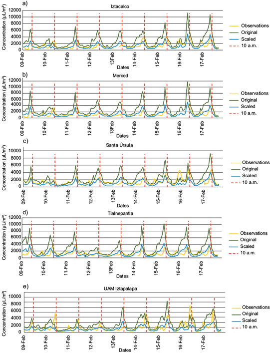
Fig. 6 Time series for the RAMA stations comparing the original and scaled modeled concentrations against measurements.
It is observed that CO concentrations are reduced when the scaling factors are applied to the original emissions. For Iztacalco, Merced, Santa Úrsula and Tlalnepantla the scaled CO concentrations are always closer to observations. As for UAM- Iztapalapa, the original concentrations are closer to observations in most of the analyzed period, but some days the scaled concentrations are closer to the measurements. This could be explained by the influence of local factors related to CO transport from other regions.
In the case of the State of Mexico stations (Fig. 7), different patterns are observed compared to the RAMA stations. For Amecameca and Ozumba, the observations are most of the time greater than the model results using either original or scaled emissions. Regarding Tenango, the original model results are closer to the observations in the hours of high concentration from February 13-15, but in other days the difference between scaled concentrations and measurements is smaller. These results suggest that most of the days CO concentrations in these sites do not originate in the MCMA; therefore, the model performance would improve only in days when there is CO coming from the MCMA.

3.5 Total column comparison
Figure 8 shows the differences in molecules cm-2 between the satellite and the model results using the original (a) and scaled (b) inventories, but also in percentage employing the original (c) and scaled (d) emissions. The greatest difference between the satellite and the model is observed when the original inventories are used and decreases when the scaled inventories are employed; therefore, these results suggest that the model performance improves after scaling the carbon monoxide emissions according to the total column comparison.

4. Conclusions
In this paper, a method was presented and applied to compare CO total columns from the WRF-Chem model and the IASI instrument, based on the methodology described by Rodgers and Connor (2003). From this comparison, scaling factors were estimated for different regions using the sensitivity characteristics of the instrument (averaging kernels) at the satellite crossing time over central Mexico. The results are important because if updated emissions are not available for a given period, they could be estimated by this method.
It is shown that the suggested method works for the IASI instrument at the analysis time reducing the difference between emissions in the 2008 emissions inventory and the current ones; therefore, the model performance improves in the surface level according to the estimated statistics (the agreement index increases up to 29% and the RMSE decreases up to 55%) and the time series (in which the scaled model concentrations approach to the observations in many cases).
Even though the concentration reported by the model is a cell of 3 × 3 km, in which several stations can exist, the model performance improves in most of the sites suggesting these types of data can be compared. The analysis may be done in higher resolution depending on the available computing resources.
It is recommended to perform the analysis over a larger period, since this would provide a greater number of comparison points; also, to include other satellite instruments such as the Tropospheric Monitoring Instrument (TROPOMI) and Measurement of Pollution in the Troposphere (MOPITT), because this would allow to analyze additional times other than 10:00 LT as well as the vertical dispersion scheme of the model, which may contribute to the attainment of different modeled vertical profiles. Since the scaling factors must always be interpreted relative to the inventory employed, in future works we suggest using other emission inventories as starting points, and then comparing the results. Since the method may be used in other modeled regions and time periods provided there are satellite measurements, it can be considered as an important tool for investigating trends and comparing different megacities.

