


 text new page (beta)
 English (pdf)
 Article in xml format
 Article references
 Send this article by e-mail
 Cited by SciELO
  Similars in
SciELO
Similars in
SciELO 
 Permalink
1. Introduction
The atmospheric high-pressure center located in the North Pacific (NPH) is closely related to the oceanographic characteristics of Southern California (USA) and Baja California, Mexico (Castro and Martínez, 2010). The NPH drives equatorward winds that maintain the eastern boundary wind-induced current known as the California Current (CC). Seasonally, wind forcing regulates the flow of the CC and determines weather patterns in the coastal areas of California and Baja California. These patterns produce two main season events: a spring-summer dry season from April to September, and an autumn-winter wet season from October to March. During the dry season, northwesterly winds induce a coastal upwelling as a known balance for the offshore Ekman divergence (Winant and Dorman 1997; Dorman and Winant 2000; Pérez-Brunius et al., 2007; Castro and Martínez, 2010; Durazo, 2015). During the wet season, the NPH weakens and migrates towards the south (Romero-Centeno et al., 2007), a process that allows low-pressure systems into California and Baja California and producing rain (Westerling et al., 2004, Hughes and Hall, 2009). Also, during this season, the relatively cold northwesterly to westerly winds dominate in the area (more than 80%) (Álvarez-Sánchez, 1977), but intense and short-lived (1 to 6 days) easterly wind events develop along California and Baja California. These events are known as the Santa Ana winds (SAw), with a typical scale of ~103 km. Their generation is associated with an intense high-pressure system in the area of the Great Basin and a low-pressure system off California, which generates strong winds. They are characterized by the dry adiabatic warming that occurs when winds flow downslope from the mountains towards the coast (Sommers, 1978; Raphael, 2003; Conil and Hall, 2006; Abatzoglou et al., 2013; Rolinski et al., 2019). Due to their nature and frequency, SAw events entirely change the climate of the coastal regions.
Over the nearby coastal ocean, the wind is particularly intensified (up to 30 m s-1) when it is channeled by canyons and creeks (Miller and Schlegel, 2006; Fovell and Cao, 2017). These easterly winds may increase ambient temperatures to ~35 °C and drastically reduce relative humidity; they may be easily identified by remotely sensed images as continental dust over the ocean, and/or smoke from forest fires (Westerling et al., 2004; Castro et al., 2006; Fovell and Cao, 2017). The meteorological events on land have been described (Hughes and Hall, 2009; Guzmán-Morales et al., 2016), and the dangers they pose are recognized through Santa Ana wind alerts (Westerling et al., 2004). Over the open ocean, SAw are associated with cold filaments shedding from the coast and changes in the productivity and optical properties (Castro et al., 2003, 2006; Trasviña et al., 2003; Sosa-Ávalos et al., 2005). However, their effects on bodies of water over the adjacent coastal ocean are less understood. This paper studies the effects of SAw over the circulation of the semi-enclosed basin of Todos Santos Bay (TSB) in northwestern Baja California. TSB, with an area of approximately 250 km2 and a mean depth of 50 m (Fig. 1), portrays a background cyclonic sea surface circulation as a response to the advection of CC water through the northern entrance (Larrañaga-Fu, 2013). Here, we hypothesize that when continental winds are present as in a SAw event, the internal circulation may also change, particularly during intense and sustained SAw events. Although numerical experiments have suggested that changes in the circulation occur during Santa Ana winds (Hernández-Walls, 1986; Argote-Espinoza et al., 1991; Mateos et al., 2009), there is a lack of field observations to support their model results, which are therefore not conclusive. In this work, we analyze the effect of SAw events on the surface circulation of TSB using hourly surface currents measured with high-frequency (HF) radar during the peak of events in the wet season over a 6-yr period.
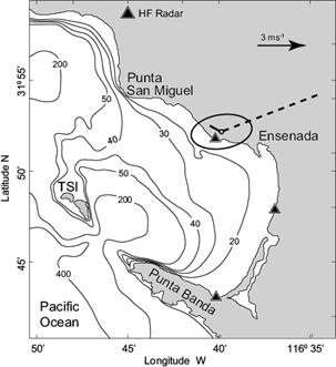
Fig. 1 Study area. Triangles show the location of sites where the high frequency radars were installed on the coast. The white circle shows the position of the weather station around which the long-term (2009-2015) wind ellipse component is drawn. Black thick line indicates the long-term wind mean direction, while broken line represents the average wind during periods of relative humidity below 35%, wind speeds > 5 m s-1 and ambient temperatures above 30 °C. Wind direction follows the meteorological convention. Contour lines indicate bottom depth (m). TSI: Todos Santos Island.
2. Data and methods
Surface ocean currents (0.5 m depth) used in this work were obtained from a high-frequency radar (HFR) network located north, east, and south of TSB (Fig. 1), operated during 2009-2015. Surface current velocities between October and March were selected for the analysis because it is during this period that the most frequent SAw events take place. However, two late SAw events that occurred during late April and mid-May 2014, were also considered. Two sets of sea surface current data were analyzed over the six-year period of this study. The first data set was obtained by a system of two radars of the “direction finding” type (~25 MHz, CODAR [www.codar.com]) (Stewart and Joy, 1974) installed in the north and east of the bay during the period October 2009 to December 2013 (Fig 1). The second set of velocity observations includes the use of an additional unit of the “beamforming” type radar (~24.5-27.3 MHz, WERA) (Gurgel et al., 1999) located in the southern region of TSB (Fig. 1), which was operational during the period from January 2013 to December 2015. In both system arrays, the radial reach was ~20 km with a spatial resolution of around 0.8 km and uncertainty of 0.06 m s-1 (Gurgel et al., 1999; Flores-Vidal et al., 2015). Current velocities calculated at each radar site provided hourly data on a Cartesian mesh of ~1 km of spatial resolution. The spatial coverage of the first array (CODAR) was represented by a regular mesh of 22 × 22 cells, while the mesh with three radars was 76 × 88, thus increasing the coverage area at the same spatial resolution. Only current speeds with a threshold value above the uncertainty were considered.
Meteorological observations were obtained using a DAVIS weather station, located north of TSB (Fig. 1). Data were referred to 10 m over the ground using a logarithmic profile. This station recorded wind data at the same times of the HF radar measurements. We contrasted these records to those obtained at Punta Morro (at different times) and found that despite minor differences in the orientation of the ellipse major axis, the DAVIS weather station reproduces the major characteristics of wind speed. Data was also consistent with regional remotely sensed wind data provided by the Cross-Calibrated Multi-Platform (CCMP) wind vector analysis product (Atlas et al., 2011; Wentz et al., 2015). Hourly wind magnitude and direction, relative humidity, and air temperatures are used here. To identify SAw events, we selected only data with relative humidity below a threshold of 45% and wind speed over 7 m s-1. This classification follows the latest SAw criteria in the southern California area (Guzmán-Morales et al., 2016).
We also used chlorophyll-a (CHL-a) images from the Ocean Colour Climate Change Initiative (OC-CCI) of the European Space Agency (oc-cci.org). CHL-a data was generated by OC-CCI by merging band-shifted and bias-corrected Medium Resolution Imaging Spectrometer (MERIS), Moderate Resolution Imaging Spectroradiometer (MODIS) and Visible Infrared Imaging Radiometer Suite (VIIRS) data with Sea-Viewing Wide Field-of-View Sensor (SeaWiFS) data. Daily images are provided with a spatial resolution of 4 km.
3. Results
The long-term mean of hourly winds measured between 2009 and 2015 in Punta Morro indicates a northwesterly wind of ~1.7 m s-1, with an ellipse component (mean ellipticity of 0.55) roughly oriented in the east-west direction (Fig. 1). The mean wind speed obtained by considering only observations when relative humidity was below 35%, speeds above 5 m s-1 and ambient temperatures above 30 °C, was 7.2 m s-1, with a direction from the northeasterly quadrant corresponding to Santa Ana winds.
Time series of meteorological variables exhibited a seasonal signal (Fig. 2). Maximum (minimum) air temperatures occur during late summer-early fall (winter) (Fig. 2a). Winter is the season when the most intense winds (~7-10 m s-1) are observed (Fig. 2b), many of them corresponding to low humidity conditions indicating the presence of northerly/easterly winds. Harmonic (annual and semi-annual) fit curves of ambient temperature explain around 54% of the total variance, with a maximum around mid-August (Fig. 2a). The corresponding value for the major axis of the wind component ellipse is 37% of explained variance, with the maximum in wind speed occurring in December-January (Fig. 2b). This wind maximum is indicated by a shift of values from negative to positive in the time series. Lastly, seasonal fits for relative humidity explain ~32% of the total variance, with minimum values in December-January (Fig. 2c). During this season, sharp drops in relative humidity (down to ~20-30 %) and increases in ambient temperature up to ~35 °C are common. These events correspond to the first quadrant easterly-northeasterly Santa Ana winds depicted in Figure 1.

Fig. 2 Time series of hourly meteorological variables recorded between 2009 and 2016. (a) Air temperature (°C), (b) major axis of the wind ellipse component (m s-1) and (c) relative humidity (%). Hourly raw data is represented by the gray line, while the red line corresponds to the 18-h smoothed raw data. The harmonic fit (annual and semiannual) of the filtered data is depicted by the black thick line. For each series, the percentage of explained variance (EV) by the harmonic fit is indicated. Dashed colored lines indicate SAw events analyzed in detail.
The frequency distribution of wind speeds during winter is shown in the wind rose of Figure 3a, which in the mean, illustrates variable and relatively weak westerly winds. This is consistent with the largest values in ellipticity observed in this season (not shown), suggesting highly variable winter winds. It also illustrates the influence of relatively strong (> 7 m s-1) northeasterly and easterly short events. Indeed, out of ~122 low humidity events recorded and identified by low relative humidity, only 27 of them (23%) exhibited wind speeds above the 7 m s-1 threshold and appeared to visibly modify the surface currents. A close view of these continental winds is depicted in Figure 3b, which indicates that although not very frequent compared to the total record in Figure 3a, first quadrant winds may be very intense (up to 12 m s-1, see also Fig. 2b).
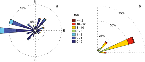
Fig. 3 (a) Distribution of wind speed and direction during winters, from 2009 to 2016; (b) same as in (a) but only for first-quadrant data with magnitude greater than 7 m s-1.
To illustrate the effect that first quadrant wind events have on the inner bay circulation, we present the winter mean currents overlaid on the detided ellipses of variability (Fig. 4). First, we separated two average winter periods of surface velocities, the times of CODAR measurements (Fig. 4a) and those measured later using phased arrays (WERA, Fig.4b). Note that WERA records showed more coverage area, due to the increased number of radar stations. Although mean currents do not exceed the range of ellipse variability, they orientate approximately in the same direction as the ellipse major axes. In general, ellipse orientations and mean currents indicate the main flow entering the bay over the northwestern opening, veering inside along the coast which suggest a cyclonic surface circulation of the bay interior, comparable to the long-term (all seasons) average currents obtained by Larrañaga-Fu (2013). Winter speeds are of the order of 5-10 cm s-1, with larger variability on the bay’s open boundary, adjacent to Todos Santos Island. Larger ellipses over the outer bay’s boundary may be associated with the variability induced by the California Current flow, although it also may be attributed to the low geophysical dilution of precision (GDOP) (Stewart and Joy, 1974). Nevertheless, data showed that variability in the bay’s interior was low, particularly near the city and port facility (Figs. 4a and b), where ellipses become more circular and of lesser size. This decreased variability is consistent with the reduced dispersion found by Cervantes-Audelo (2014) in the same region.
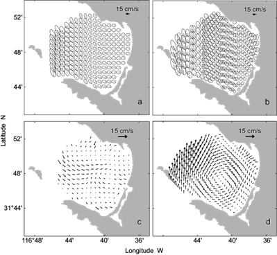
Fig. 4 Low pass filtered surface current ellipses of variability for Todos Santos Bay. (a) Winters from 2010 to 2013 obtained with two CODAR radar systems; (b) winters from 2014 to 2016 obtained with WERA radar systems. Lines with origin at the center of ellipses represent the average winter current. (c) Average surface currents obtained by considering only the times of Santa Ana wind events during the CODAR instrument setup; (d) same as (c) but for the WERA systems. Note that in (b) and (d), about 50% of the original coverage is shown for clarity.
For both winter periods of Figure 4a, b, we extracted and averaged surface currents measured during selected (> 7 m s-1) first quadrant wind events. The resulting patterns are shown in Figure 4c, d for CODAR and WERA measurements, respectively. Surface currents obtained with CODAR were calculated using nine events (Fig. 4c). Average surface currents during these periods depicted two eddies, cyclonic in the north and clockwise in the south, converging around the center of the bay. Over the TSB open boundary, surface velocity was slightly larger than inside the bay and had the same direction as the CC flow observed in the long-term mean (Larrañaga-Fu, 2013). In contrast, surface currents obtained from the records of four events during WERA measurements (Fig. 4d) depicted an anticyclonic eddy covering most of TSB. The open boundary surface velocities were larger and had opposite direction to that of the CC flow there. Inside TSB, surface currents were slightly stronger than the winter average shown in Fig. 4b, likely caused by the stronger winds (~12 m s-1) during the WERA measurement period. A flow parallel to the coast was also observed, bonding the large vortex around the bay.
Differences in surface circulation patterns between the two winter periods may be attributable to differences in the particular response of surface waters to each Santa Ana wind event. To analyze particular responses, we selected three periods of strong first-quadrant winds and obtained the average resulting surface currents. The first SAw event selected occurred on December 14-21, 2011 (Fig. 5), when the main wind direction was northeasterly, with wind speeds ranging from ~2 to above 10 m s-1 (Fig. 5a). Event-average surface currents depicted a flow towards the west-northwest (Fig. 5b), although not very intense, mainly along the northern and southern coasts. At the start of the event, relative humidity drastically reduced from ~70 to ~30% (Fig. 2c). Other than a change in the direction of surface currents (not shown), there was not a clear signal of currents to intensify in response to the forcing winds, possibly due to the effect of the constrained bay and its shallow bathymetry that apparently controlled their intensity during this event.

Fig. 5 SAw event for December 14-21, 2011. (a) Wind speed and frequency during the period. (b) Mean surface currents. Arrows indicate speed and direction, while color contours show the velocity root mean square. The open circle indicates the position where time series of surface currents is extracted. (c) Time series of smoothed wind speed (blue line, m s-1), relative humidity (green, %) and average surface current velocity (red, cm s-1). The latter was obtained at the location shown by the open circle in (b).
Another SAw event occurred between April 29 and May 4, 2014 (Fig. 6). As the previous one, the event was characterized by the sharp drop in relative humidity, from 80% to less than 10%, in a matter of hours. Moderate to intense (4-8 m s-1) first quadrant winds (bursts of 8-10 m s-1, Fig. 6a) forced the flow offshore over the bay’s southwestern region, with maximal velocities of 35 cm s-1 between the island and the continent (Fig. 6b). Over the inner bay, currents changed direction relative to the mean winter circulation, and intensified mainly along the southern area of TSB (Fig. 6c), reaching values up to 50 cm s-1. Current speed intensification matched the SAw intensification and flow direction (not shown) during the three days of the event. However, currents did not display a clear diurnal signal as did wind speed.
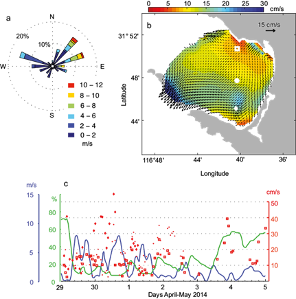
Fig. 6 Same as Figure 5 for April 29 to May 5, 2014. Symbols for surface currents correspond to the locations indicated in (b).
The third case presented occurred a few days after the previous event, in May 11-15, 2014 (Fig. 7). Dominant winds observed were easterly and northeasterly, with maxima of ~12 m s-1 and bursts up to 15 m s-1(Fig. 7a). The average circulation pattern depicted a clockwise circulation centered over the southern half of the bay, with a relatively strong (~30-40 cm s-1) northward flow over the open boundaries (Fig. 7b). The event evolved after a sharp decrease in relative humidity, during the first three days (Fig. 7c) from 80% to less than 10%. Contrasting to the two previous events described, surface currents not only changed direction (to overturn the mean winter cyclonic circulation suggested in Fig. 4), but also intensified, especially during the first three days of the event in the three locations selected along a north-south transect. Similar to the previous event of April 29 to May 4, 2014 (Fig. 6), wind speed showed a diurnal signal likely related to the daily strengthening of the coastal-ocean changing horizontal pressure gradients. However, the diurnal intensification on surface currents was not clearly observed, although maximum current speeds up to 60 cm s-1 followed peaks in wind speed (Fig. 7c). This damping of the diurnal signal under very intense easterly winds was also observed by Castro et al. (2006) in records of sea surface temperature.

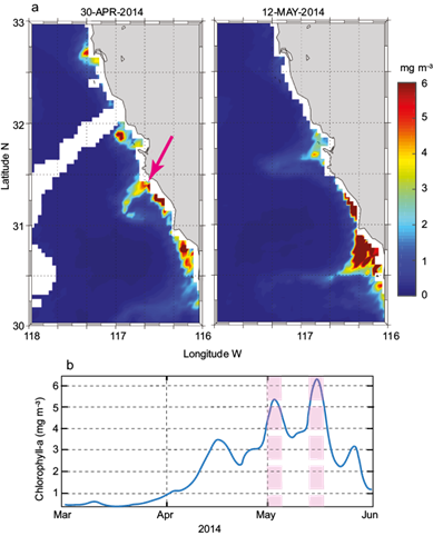
The examples provided suggest that during strong easterly-northeasterly wind events, surface water is transported outside TSB. Besides the vertical mixing promoted by the strong winds, this offshore transport might generate a mechanism to promote upwelling in the coastal regions by the replacement of the recently displaced water from underneath and hence, an increase in the concentration of nearshore chlorophyll-a, as has been previously suggested (Castro et al., 2006). Such coastal increase is observed in the satellite images of April 30 and May 12, 2014 (Fig. 8a), and also revealed in the time series of this variable at a coastal location (Fig. 8b). High values of nearshore chlorophyll-a may be attributable to the peak of the upwelling season from March to June (de la Cruz-Orozco et al., 2017). However, noteworthy are the chlorophyll-a increases (1-2 mgm-3) related to the times of intense first-quadrant winds in April and May. These increases and the wind direction may add in the process of transporting recently upwelled waters into the open ocean, as is suggested by the high-productivity filaments in the satellite images.
4. Discussion
The effects of easterly-northeasterly Santa Ana winds on the background surface circulation of Todos Santos Bay (TSB) is described. Previous works using drifting buoys during short-timed experiments (hours) have suggested that surface currents may rapidly veer towards the same direction as the wind when SAw occur in the area (Álvarez-Sánchez, 1977; Álvarez-Sánchez et al., 1988; Durazo-Arvizu and Álvarez-Sánchez, 1988). However, the limitations of such experiments (drifting buoys positioned by X-radar) were not conclusive and did not allow to study the response over longer times because the increase in sea surface roughness prevented buoy positioning during strong winds (Álvarez-Sánchez et al., 1988). This change of direction has also been suggested in numerical simulations when SAw scenarios were included as initial forcing (Hernández-Walls, 1986; Argote-Espinoza et al., 1991). In the present work, the high temporal and spatial resolutions (1 h, 1 × 1 km) sea surface current data obtained in the period 2009-2015 allowed us to isolate conditions during specific times and document the changing currents in response to the acting winds during easterly wind events. We observed a change in rotation from the winter-mean cyclonic patterns observed for NW and W winds (Fig. 4a, b), to an anti-cyclonic rotation (Fig. 4c, d) during SAw. Two outcomes can be summarized from our study. One is that the surface circulation resulting from the SAw forcing was not always the same, and another is that regardless of the resulting circulation during SAw, offshore transport of surface waters was observed.
The fact that sea surface current patterns differ for each SAw event may be related to the direction in which winds blow and their intensity on a particular case. Scrutiny of Figures 2 and 3 (and wind direction records, not shown) indicates that some SAw events enter from the northeast and other from the east (with maximum wind intensities), guided apparently by the spatial distribution of the regional high-pressure center (Raphael, 2003) and by the two main topographical depressions over land, which in great measure may determine the direction of the incoming wind (Álvarez-Sánchez, 1977). A similar relationship between SAw events and surface currents in the ocean has also been observed in California, USA, as winds are guided by coastal depressions (Hu and Liu, 2003; Rolinski et al., 2019). Thus, at varying speeds and directions at which SAw events occur, we could expect a different sea surface current pattern to occur. This is especially true given the fact that HF radars measure less than the first meter of the sea surface, that is, where the maximum momentum transfer between the atmosphere and the ocean takes place. This would imply this thin layer would closely follow the direction of the forcing wind. Further development of the inner circulation is likely modulated by bathymetry and coastal configuration, such that rather strong easterly winds may generate an overturn of the background circulation, as was observed in May 11-15, 2014 (Fig. 7). While our measurements cannot fully establish a direct relationship between wind intensity/direction into the resulting surface currents pattern, it does give a guide into additional scenarios that may be considered when using numerical simulations to study the response to regional forcings.
Average current maps during moderate to strong SAw events suggested an offshore transport of surface waters (Figs. 5-7). This process has important implications in the renovation of internal waters. Offshore advection of surface waters by wind may be an efficient ventilation mechanism through which the inner bay is sanitized since it promotes the exchange of inner waters with the open ocean, at least during the duration of easterly wind events. In a statistical analysis of surface currents of TSB, Cervantes-Audelo (2014) found that the background cyclonic circulation of the bay implies longer residence times in regions close to the city port and beaches, thus elevating the risk of concentrating elements near populated areas. By forcing water out of the bay during SAw, we could expect an improvement in the water quality of the coastal areas and inside TSB, as surface water may be exchanged vertically by turbulence and entrainment, and horizontally by advection. Evidences of the displacement of coastal waters offshore is provided by the minimal values in sea surface temperatures regularly observed nearshore during SAw events (Hu and Liu, 2003; Trasviña et al., 2003; Castro et al., 2006) and by the increase of CHL-a in the coastal region (Hu and Liu, 2003; Sosa-Ávalos et al., 2005; Castro et al., 2006). Figure 8 depicts daily satellite CHL-a images for two cloud-free days during the SAw events of April 30 and May 12, 2014. In both images, maximum concentrations (> 5 mg m-3) are observed inside TSB and at coastal locations outside (Fig. 8a, b). While the high CHL-a concentrations may be attributed to coastal upwelling due to the offshore Ekman transport typical of the season (Durazo, 2015), time series at a fixed point (Fig. 8c) suggest that important increases in CHL-a may be associated with SAw events. Peak values in CHL-a are observed around the same times peak easterly wind speeds occur. Besides, color images illustrate the presence of filaments transporting high-nutrient water to the open ocean. Thus, SAw not only modify the background circulation inside the bay but also promote its ventilation by the offshore transport of enriched waters.
Several aspects of inner bay kinematics and dynamics, not possible to elucidate with our present data, still remain to be settled. For example, once a change in circulation and the offshore transport are established during a SAw, there also should be changes in the three-dimensional circulation produced to achieve mass balance. A recent study by Flores-Vidal et al. (2018) has shown that cross-bay subsurface transports at the bay’s entrances may be controlled by friction and kinematics. Thus, we could expect that changes in the circulation related to intense easterly winds and the intensification of surface currents, as observed in this work, could notably modify the way water is exchanged below the surface. While these results shed some light in the likely exchange processes that may occur, they are not conclusive. Certainly, more research is needed to elucidate the variability in the mechanisms of transport across the bay entrances.
Another aspect that requires further consideration is the study of residence times of inner water. Although data suggests residence times can be drastically reduced under easterly wind forcing, more work is also needed to investigate not only horizontal gradients in oceanic variables resulting from the forcing, but also the air-ocean heat exchanges (expected to be extreme in latent heat loss; see Castro et al., 2006) that can drastically modify such residence times (Graham and Largier, 1997). Ultimately, the goal would be to discern how these processes and mechanisms aid in the healthiness of TSB (as has been pointed out by Ramírez-Álvarez et al., 2020), a critical aspect for a semi-enclosed water body that is under an increased stress due to the demanding growing population.
5. Concluding remarks
Seven years of winter-season surface current measurements inside Todos Santos Bay revealed that different responses in the circulation occur under the influence of varying northeasterly-easterly Santa Ana winds. Such responses generally include a change in the direction water flows. Under the influence of extreme easterly winds (> 10 m s-1), the winter-mean circulation pattern may overturn from cyclonic to anti-cyclonic. Largely, deviations from the long-term mean patterns comprise an offshore transport of surface waters into the open ocean. These results emphasize the importance of using novel technology for surface current measurements at high time and spatial resolution, and provide a robust tool to gather new insights of the kinematics and dynamics of the inner bay, aimed at solving problems not previously addressed by conventional methods, such as dispersion of particles, and mixing and transfer of properties between coastal embayments and the open ocean.

