


 nueva página del texto (beta)
 Inglés (pdf)
 Artículo en XML
 Referencias del artículo
 Enviar artículo por email
 Citado por SciELO
  Similares en
SciELO
Similares en
SciELO 
 Permalink
1. Introduction
In recent decades, hydrological models have become increasingly useful and important tools in water resource planning and management. Various hydrological models have been developed to simulate hydrological processes in a watershed. These models include:
Simple models such as the Soil Conservation Service (SCS), NAM (Nielsen and Hansen, 1973), TANK (Sugawara, 1974), TOPMODEL (Beven and Kirkby, 1979), Identification of Hydrographs and Components for Rainfall, Evapotranspiration and Stream Flow Data (IHACRES) (Croke et al., 2003).
Complex models such as MIKE-SHE (Refsgaard and Storm, 1995), WetSpa (Wang et al., 1997) and the Soil and Water Assessment Tool (SWAT) (Arnold et al., 1993).
Both the SCS (USDA, 1972) and SWAT models were developed by the U.S. Department of Agriculture (Arnold et al., 1993). Selecting the most appropriate model from this broad array of options depends on watershed characteristics and management goals (Borah et al., 2006; Liu, 2018) as well as available data (Croke and Jakeman, 2008; Lobligeois et al., 2014). With increasing model complexity, the cost of implementing the model increases (Croke and Jakeman, 2008). Therefore, in selecting a suitable model, many factors come into play.
In watersheds with scarce data, simple watershed-scale models are often preferred to complex models, as the former require less data. However, simple models may not generate desirable outputs, while complex models are inappropriately complex and could be prohibitively expensive to implement in large watersheds (Borah et al., 2006). Selecting a suitable hydrologic model for a given purpose and a specific watershed requires a trade-off between model complexity and data availability. Complex models require detailed databases containing information on phenomena such as groundwater delay, initial roughness after last tillage, hydraulic conductivity through pond bottoms, and organic nitrogen concentration in the channel, data that are often not available. In general, the best model for a specific watershed is the one which gives results as close to reality as possible, with the use of the least number of parameters and model complexity (Ha et al., 2017).
Some studies have shown that decreasing spatial resolution did not have a significant effect on model performance in streamflow simulation (Das et al., 2008; Apip et al., 2012). Other studies have shown that the results of streamflow simulation can change significantly due to the spatial heterogeneity of rainfall patterns (Koren et al., 2004; Arnaud et al., 2011; Apip et al., 2012). Information on spatial and temporal variations in rainfall is therefore important in understanding hydrological processes (Lobligeois et al., 2014).
In arid and semi-arid climates, rainfall depth is low but its intensity usually high. In these areas, heavy rainfall leads to a rapid hydrographic response, with higher peak discharges (Croke and Jakeman, 2008; Golshan et al., 2016). In contrast, in humid areas the response to rainfall is very slow and peak discharge takes more time to occur (Ward, 2003). Such differences in climate can be expected to have a large impact on the performance of streamflow simulation models.
The hydrological models used in this study are commonly employed and were selected due to their widespread use in Iran and other countries (Taesombat and Sriwongsitanon, 2010; Tho et al., 2016; Islam et al., 2017). We selected simple watersheds in Iran with three different climates where running different models can give information about their performance in diverse regions of a country.
Accordingly, the main objectives of the present study were to: (i) analyze the sensitivity of model parameters for different climates, (ii) compare flow characteristics for these climates, and (iii) assess the feasibility of using SWAT and IHACRES models to simulate flow discharge in three completely different climate zones in Iran.
2. Study areas
Three climates are dominant in Iran (Zareiee et al., 2014). In the central and southern regions of Iran, arid climate is dominant due to its latitude and proximity to a subtropical high-pressure region (Alijani, 1997). Table I shows altitudinal, latitudinal and longitudinal ranges, annual mean precipitation, runoff and temperature, as well as Köppen climate classification system designations for three watersheds: Jazmurian (arid;W arid ), Khorramabad (semi-arid; W sa ), and Talar (semi-humid; W sh ), located in southern, central and northern Iran, respectively. The three watersheds, each from a different climatic region, are presented in Figure 1. A vast range of data is needed for running models in these selected watersheds, which have better data than other watersheds in the same climatic regions. The normality and homogeneity of the data were assessed and a common statistical period was selected as models input.
Table I Characteristics of the arid, semi-arid and semi-humid watersheds under study.
| Site | Area (km2) | Elevation (masl) | Location | Measured annual means | Climate | ||||
| P (mm) | T (Cº) | R (mm) | |||||||
| W arid | 1258 | 1969 | 3798 | Kerman (South) | Jazmurian | 162 | 22 | 33.35 | Arid |
| W sa | 2267 | 949 | 2981 | Lorestan (Central) | Khorramaban, in Karkheh basin | 402 | 15 | 68.77 | Semi-arid |
| W sh | 2057 | 216 | 3977 | Mazandaran (North) | Talar, in Haraz basin | 609 | 11 | 153.31 | Semi-humid |
P: precipitation; T: temperature; R: runoff.
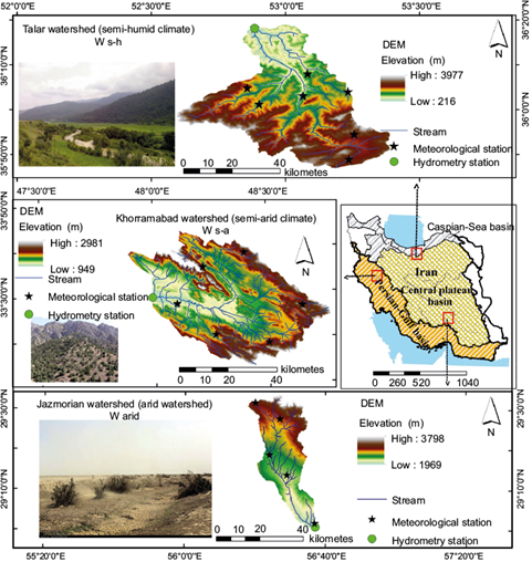
Climates of the study areas were classified according to the Köppen climate classification system (Table I) (Djamila and Yong, 2016).W arid is characterized by dry land agriculture with poor soil fertility. In W sa , most precipitation occurs in December and April, and rangelands and natural environment have a better condition than in W arid . Dense bushes cover many parts of the W sa area. This last watershed is located along the southern coastline of the Caspian Sea, and is categorized by warm, humid summers and conditions suitable for agriculture.
3. Methodology
3.1 Description of the SWAT model
The SWAT model is a physically based, comprehensive, continuous, semi-distributed and watershed-scale simulation model that can simulate most of the hydrological processes in watersheds (Arnold et al., 2012; Islam et al., 2017; Kavian et al., 2017). Primary input data for the SWAT model comprises land use data, a digital elevation map, a soil texture map and meteorological records. The SWAT model divides a catchment into sub-catchments and then further divides each sub-catchment into smaller homogeneous units known as hydrologic response units (HRU), based on unique combinations of land use, soil class and land slope (Neitsch et al., 2011; Pirnia et al., 2018).
The simulation of the hydrological cycle by SWAT is based on the water balance equation, presented as follows:
where SW t is the final soil water content (mm), SW is the initial soil water content on day i (mm), t is time (days), n is the total number of days, R t is the amount of precipitation on day i (mm), Q t is the amount of surface runoff on day i (mm), ET t is the amount of evapotranspiration on day i (mm), P t is the amount of percolation on day i (mm) that may reach to the underground water, and QR t is the amount of return flow on day i (mm).
In the SWAT model, surface flow can be simulated using two methods: (i) the Soil Conservation Service (SCS) Curve Number (CN) and (ii) the Green-Ampt infiltration (Neitsch et al., 2011). The SCS method was applied in this study with surface flow rate calculated as follows (Bosznay, 1989):
where, Q surf is the accumulated runoff (mm), R day is the rainfall depth for the day (mm), and S is the potential maximum soil moisture retention after runoff begins (mm). Daily mean rainfall was calculated, in each case, using the skewed normal option. To calculate potential evapotranspiration, three methods are available: Penman-Monteith, Priestley-Taylor, and Hargreaves. In this study, the Hargreaves method was used (Eqs. 3 and 4, Neitsch et al., 2005). Actual evapotranspiration was then derived from potential evapotranspiration as a function of plant parameters and water storage in the soil (Neitsch et al., 2011).
where ET o is evapotranspiration (mm), K t is an empirical constant calculated using Eq. (4), R a is the water equivalent of extraterrestrial radiation (MJ d-1), calculated based on the latitude of the site and the specific month when data is collected, TD is the average difference between maximum and minimum temperatures for day i, and T is the average temperature on day i (ºC).
3.2 Calibration, validation and uncertainty of the SWAT output
SWAT-CUP is a program developed by Abbaspour et al. (2007) to automatically assess sensitive model parameters and calibrate SWAT by optimizing parameter values. In this study, integrated algorithm consecutive uncertainty (SUFI2) was selected for simulation because it has the potential to change and analyze parameters with the lowest number of model repetitions (Ha et al., 2017). The global sensitivity analysis option of the SUFI2 program was applied for sensitivity analysis and uncertainty analysis. In the parameters sensitivity analysis and calibration step the SUFI2 algorithm was performed in 350 and 1000 repeats. Among various evaluation coefficients available in SUFI-2, the Nash-Sutcliff model efficiency coefficient (NS) was selected for model calibration in SWAT-CUP. In order to analyze uncertainty and determine 95% prediction uncertainties (95PPU), the SUFI2 algorithm uses p-factor and r-factor (Abbaspour et al., 2007). The p-factor is a percentage of observed data bracketed by the 95% prediction area known as 95PPU. In the other hand, the r-factor is the average width of the 95PPU band divided by the standard deviation of the measured variable. More detailed information on the process to create a SWAT-CUP program, specifically SUFI2, are available in Abbaspour et al. (2007).
3.3 Description of the IHACRES model
The IHACRES model (Jakeman et al., 1990) is a watershed-scale rainfall-runoff model that was developed for semi-arid Australian watersheds. This model was updated to version 2.1 by the Centre for Resource and Environmental Studies (CRES) of the Australian National University (Taesombat and Sriwongsitanon, 2010). Its purpose is to assist the hydrologist or water resources engineer to characterize the dynamic relationship between basin rainfall and streamflow (Croke et al., 2005). We chose the IHACRES model because it is applied throughout the world and has been recently applied with success (Samuel et al., 2011; Sriwongsitanon and Taesombat, 2011; Onyutha, 2019). One of the major advantages of this model over other hydrological models is the minimal data input requirement (Zolghadr-Asli et al., 2018). It engages either linear, nonlinear, or multiple regression methods to estimate streamflow (Jakeman et al., 1990; Samuel et al., 2011). The effective rainfall u k in the revised model, which must be nonnegative, is given by (Wheater et al., 2007):
where r k denotes the measured rainfall (mm), c denotes the water balance coefficient, l represents the soil moisture index, p denotes the power of the soil moisture index, and Φ k is the soil moisture index. Evapotranspiration is a valuable parameter for obtaining soil moisture and effective rainfall, and is calculated as (Croke and Jakeman, 2004):
where E T,k , M k , and T k are evapotranspiration, catchment moisture deficit, and temperature for time step k, and c 1 and c 2 are parameters affected by rainfall depth for time step k.
The flow concentration calculation module converts u t into discharge and simulate the peak flow response and flow recession process. The following equations are relevant (Kan et al., 2016):
where L is the lag time step, X t s and X t q are slow and quick discharge, respectively, α s and α q represent the recession rate of slow and quick discharge respectively, and β s and β q are the peak flow response of slow and quick discharge, respectively.
Dynamic response characteristics (DRCs) unit hydrographs for quick flow and slow flow are respectively calculated as (Taesombat and Sriwongsitanon, 2011):
where ∆t is the computation time step (daily), α q and α s are time constants, and τ q and τ s are the recession time constants for quick flow and slow flow in days, respectively. The parameter τ q ranges between 0 and 5 (Kan et al., 2016). The relative volume of quick flow and slow flow can be calculated as (Taesombat and Sriwongsitanon, 2011):
where V q is the proportion of quick flow to total flow (1 - V s ), and β q and β s are the peak flow response of slow and quick discharges (m3 s-1), respectively. This version of the non-linear module is described in detail in Jakeman et al. (1990) and Jakeman and Hornberger (1993).
3.4 Calibration and validation of the IHACRES output
A large number of software frameworks have been developed for optimizing the lumped model parameters using the open-source R software. In this study, the Hydromad package was used to optimize the IHACRES model parameters. This package provides a set of functions to perform the model in large repetitions. The details of this package can be found online at http://hydromad.catchment.org/. Several optimization algorithms are available for calibrating the models that the DEoptim (Price et al., 2005) was used in this study. To simulate the streamflow, rainfall, temperature, and observation streamflow values were entered in the algorithm and performed in 500 repeats. Finally, the optimum value for each parameter in different climates was obtained and used for the IHACRES model simulation.
3.5 Preparing data and simulation streamflow
The input data used in the SWAT model can be broadly categorized into three groups for model calibration: spatial data, climate data and flow data.
3.5.1 Climate and flow data
Accordingly, towards the goal of running the model in each distinct climate we selected watersheds (W arid , W sa , and W sh ) for which a complete and accurate database was available. Climate data consists of a weather generation (WGN) table, daily rainfall, daily minimum and maximum temperatures, daily mean wind speed and daily mean relative humidity. The number of used meteorological stations inW arid , W sa , and W sh are eight, six and five, respectively (shown in Figure 1). All stations are active and could provide long term data. The data sets were checked for normality and homogeneity by using parametric and nonparametric tests. Rainfall, temperature, wind speed, humidity and radiation over a 20-year period were used to prepare the WGN table. As inputs, the SWAT model receives weather station names, elevation, and geographical coordinates. The skewed normal method was used to calculate daily rainfall.
3.5.2 Spatial data
Spatial data consisted of a digital elevation map (DEM), a soil texture map, and a land use map, all prepared at a 28-m cell resolution. To prevent the creation of an unnecessarily large number of HRUs, the threshold for HRU creation was set at 10% of the total sub-basin area. Daily streamflow data were obtained from hydrometric stations at the outlets of each of the three watersheds. The mean observed streamflow in theW arid , W sa , and W sh watersheds was 1.33, 5.84, and 8 m3 s-1, respectively. Using the observed mean discharge and precipitation, the percent of precipitation lost by evapotranspiration was calculated as follows:W arid ,79.41%; W sa , 77.23%; and W sh , 74.82 %. The period from 2000-2010 was selected for models’ calibration in each watershed. In addition, data spanning the three-year period of 1997-1999 served to warm up the SWAT model. The validation period for all watersheds was 2010-2015. The IHACRES model used climate data and streamflow with daily steps as input data (Table II). Both models required a watershed area value for determining the amount of output discharge.
Table II Source of input data for the SWAT and IHACRES models.
| Source | Description | Data |
| River flow | Jazmurian hydrometric station Khorramabad hydrometric station Talar hydrometric station | Kerman Regional Water Company Lorestan Regional Water Company Mazandaran Regional Water Company |
| Meteorology | Talar: stations Baladeh, Chamestan, Edareh Babol, Firozkoh, Gatkola, Kadir and Karesang Khorramabad: stations Cham Angi, Dehno, Kakareza, Khorramabad, Srabsy and Sorkhab Jajmoreian: Bydkrdvyyh, Jamil Abad, Baft, swch, Kigan | Regional Water Company and Meteorological Department of the Province |
| DEM | 12.5 ×12.5 m | https:/doi.org/vertex.daac.asf.alaska.edu/ |
| Land use | W arid : 7 land use types W sa : 11 land use types W sh : 7 land use types | Department of Natural Resource and Catchment Management |
| Soil map | W arid : clay, loamy, silty W sa : clay, clay-loam, sandy- clay-loam, sandy-loam W sh : clay, clay-loam, loamy, silty, silty-loam | Regional Water Company |
3.6 Evaluation of model performance
To evaluate model performance, several statistical indicators must be determined (Santhi et al., 2001; Gassman et al., 2007). In the current study the Nash-Sutcliffe model efficiency coefficient (NS), the regression coefficient (R2) for the linear relationship between measured and modelled values, the percent bias (PBIAS), and the deviation of discharge (D v ) were used to quantitatively assess model performances in simulating monthly streamflow. The range of values for the R2 and NS coefficient are between -1.0 to 1.0 and -∞ to 1.0, respectively. In these coefficients, values equal to 1.0 represent a perfect fit simulation, and values near to 1.0 show a fit simulation (Kavian et al., 2017). The optimal value for PBIAS is 0.0, since low-magnitude values show precision simulation. Positive and negative values in these criteria indicate overestimation and underestimation, respectively (Islam et al., 2017). The other used criteria for assessing the model performance was D v . Donigian et al. (1983), Singh et al. (2005) and Wu and Johnston (2007) indicate that in terms of model simulations D v < 10% can be considered very good, 10% < D v < 15% good, and 15% < D v < 25% fair.
where Q
i
obs
is the i
th
observed discharge, Q
i
sim
is the i
th
simulated discharge,
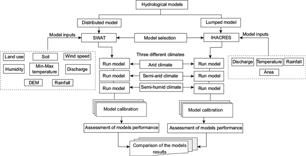
The flowchart in Figure 2 illustrates complex and simple models for the three different climatic areas.
4. Results and discussion
For the SWAT model, the watersheds under study were divided into sub-watersheds, resulting in 8, 33 and 23 sub-watersheds forW arid , W sa , and W sh , respectively. The sub-watersheds were further partitioned into HRUs, which were based on unique overlays of land use, land slope and soil type layers. After overlapping these layers, 96, 223 and 265 HRUs were created in theW arid , W sa , and W sh watersheds, respectively.
4.1 Flow discharge simulation results
4.1.1 SWAT model calibration
The results of the sensitivity analysis for the SWAT model using the SUFI2 algorithm are presented in Table III. In each watershed, the most sensitive parameters were selected for model calibration. The number of parameters used for the calibration of the SWAT model were limited to prevent over-parameterization. The most sensitive parameter for all three watersheds was CN2, implying that this parameter was sensitive to different climates. This was consistent with previous studies in Iran (Ghobadi et al., 2015; Dowlatabadi and Zomorodian, 2016; Gholami et al., 2016). The rank of sensitivity for the parameters was different for each watershed. The parameters of soil evaporation compensation (ESCO), groundwater delays (GW_DELAY) and available water capacity of the soil layer (SOL_AWC) were sensitive for watershedW arid . The alpha coefficient for the baseflow recession curve and ALPHA_BNK were sensitive only for watershed W sa . Similarly, saturated hydraulic conductivity (SOL_K) and surface flow lag time (SURLAG) were only sensitive parameters in the case of watershed W sh . This suggests that the sensitive parameters in semi-arid and semi-humid watersheds are more alike than implied by Tho et al. (2016). The set of seven most sensitive parameters was unique for each watershed. Initial ranges for each parameter and final calibrated values via the SUFI2 algorithm are shown in Table IV.
Table III SWAT model sensitivity analysis results.
| (W sh ) | (W sa ) | (W arid ) | Comments | Parameters |
| Sensitivity rank | ||||
| 1 | 1 | 1 | Initial SCS runoff curve number | CN2 |
| - | 2 | - | Baseflow alpha factor for bank storage (day) | ALPHA_BNK |
| 2 | - | - | Saturated hydraulic conductivity (mm h-1) | SOL_K |
| 3 | 3 | 5 | Deep aquifer percolation fraction | Rchrg_Dp |
| 5 | 4 | 2 | Threshold depth of water in the shallow aquifer required for return flow to occur (mm) | GWQMN |
| 4 | 5 | - | Soil depth (mm) | SOL_Z |
| - | 6 | 4 | Manning coefficient in the main river | CH_N2 |
| 6 | 7 | - | Groundwater revap | REVAPMN |
| 7 | - | - | Surface flow lag time (days) | SURLAG |
| - | - | 3 | Soil evaporation compensation factor | ESCO |
| - | - | 6 | Available water capacity of the soil layer (mm H2O/mm soil) | SOL_AWC |
| - | - | 7 | Groundwater delay (days) | GW_DELAY |
Table IV Initial parameter calibration ranges and calibrated parameter values for the SWAT model in three watersheds.
| Talar (W sh ) | Khorramabad (W sa ) | Jazmurian (W arid ) | Parameters | |||
| Calibrated value | Initial range | Calibrated value | Initial range | Calibrated value | Initial range | |
| 0.67 | (-0. 695-0.751) | 0.337 | (-0.3-0.762) | -0.71 | (-0. 8-0.8) | r-CN2 |
| 1.149 | (-0.54-2.63) | 0.083 | (-0.562-0.58) | - | - | v-ALPHA_BNK |
| 0.567 | (-0.0053-0.748) | - | - | - | - | r-SOL_K |
| 0.016 | (-0.047-0.624) | 0.428 | (0.086-0.5) | 0.39 | (0- 1) | v-Rchrg_Dp |
| 0.537 | (0.09-1.794) | 0.93 | (0.017-1.219) | 0.374 | (0.06-1.126) | r-GWQMN |
| 0.604 | (0.326-1.362) | 0.534 | (0.243-1.927) | - | - | r-SOL_Z |
| - | - | 0.418 | (0.017-1.562) | 0.283 | (0.054-1.36) | v-CH_N2 |
| 0.198 | (0.06-0.621) | 0.134 | (0.145-0.446) | - | - | v-REVAPMN |
| 1.234 | (-0.144-1.57) | - | - | - | - | v-SURLAG |
| - | - | - | - | 0.58 | (0-0.975) | r-ESCO |
| - | - | - | - | 0.301 | (0.215-0.771) | r-SOL_AWC |
| - | - | - | - | 21 | (0-100) | v-GW_DELAY |
r-: multiply existing value by obtained absolute value (+1); v- : replace existing value with calibrated value (Kavian et al., 2017).
4.1.2 IHARES model calibration
Calibrated values for the IHACRES model parameters inW arid , W sa , and W sh are summarized in Table V. All the IHACRES parameters have an important effect on simulated streamflow in the watersheds; however, the relative volume of the slow flow parameter has the highest sensitivity and the mass balance parameter (c) the lowest. This concurs with the results of Taesombat et al. (2010). Calculating the DRCs’ unit hydrographs for quick flow and slow flow in different climates resulted in a higher value for the arid watershed (W arid ) compared to the humid watershed (W sh ). This suggests a higher likelihood of flash floods in arid areas (Knox, 1985). The soil moisture parameter (τ w ) increased from the arid to the humid climate, whereas parameter c decreased. These results are similar to those found in Sriwongsitanon and Taesombat (2011) for semi-humid and humid areas.
Table V Calibrated parameters for the IHACRES model.
| Linear module | Non-linear module | Hydrometric stations | ||||
| V s | τ q | τ s | f | τ w | c | |
| 0.53 | 2.64 | 69.87 | 0.33 | 1.02 | 0.091 | Jazmurian (W arid ) |
| 0.86 | 2.03 | 41.54 | 0.63 | 1.27 | 0.002 | Khorramabad (W sa ) |
| 0.74 | 1.226 | 33.52 | 1.59 | 6.16 | 0.00075 | Talar (W sh ) |
τ s : recession time constant for slow flow in days; τ q : recession time constant for quick flow in days; V s : relative volume of slow flow; c: mass balance; τ w : soil moisture; f: temperature coefficient.
4.2 Model performance assessment for three different climates
Discharge rates in the three watersheds were simulated using the SWAT and IHACRES models for the period of 2000-2010 (Fig. 3). In the model calibration and validation stages, concordances between observed and simulated streamflow (at monthly time steps) were evaluated using statistical and graphical measures. The simulated streamflow for both models and R2 coefficients are shown in Figure 4. According to Motovilov et al. (1999), simulation of the hydrological model can be considered good if R2 > 0.75 and satisfactory if R2 is between 0.36 and 0.75.
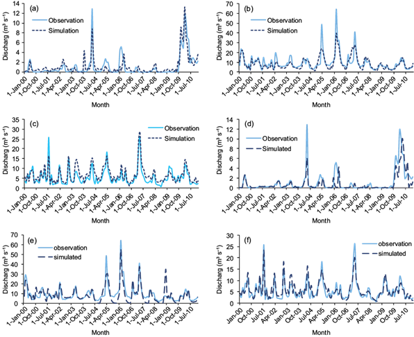
Fig. 3 Observed and simulated discharge during the calibration period using the SWAT model (at monthly time steps): (a) Jazmurian, (b) Khorramabad, and (c) Talar; and the IHACRES model: (d) Jazmurian, (e) Khorramabad and (f) Talar.
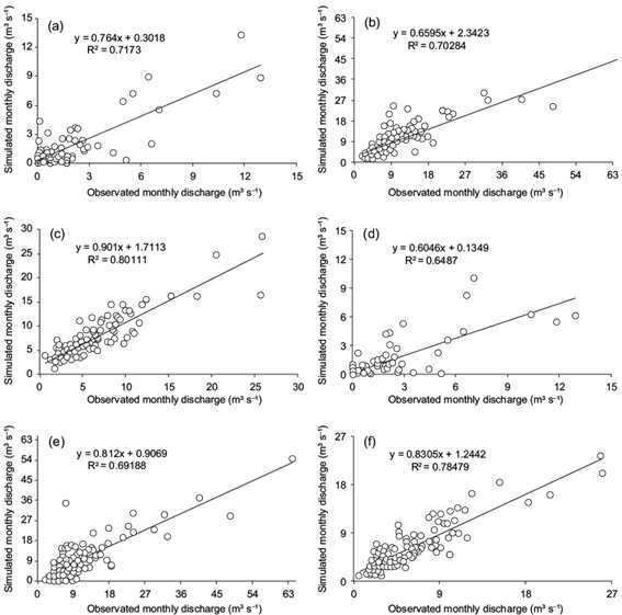
Fig. 4 Correlation between observed and simulated discharge during the calibration period using the SWAT model: (a) Jazmurian, (b) Khorramabad, and (c) Talar; and the IHACRES model: (d) Jazmurian, (e) Khorramabad, and (f) Talar.
The uncertainty analysis was also performed for SWAT model outputs using the p- and r-factors in the SWAT-CUP model. The calculated values for these criteria are listed in Tables VI and VII. A balance between the p- and r-factors is observable, and the parameter ranges of both factors reached the desired limits. The r-factor is less than 1 in all stations both in the calibration and the validation period, which generally shows a good calibration result (Kavian et al., 2017). In the other hand, the p-factor is near to 1 in all stations, which indicates that uncertainty in the simulation results is lower.
Table VI Assessment of the SWAT and IHACRES models performance during the calibration period.
| r-factor | p-factor | Dv (%) | PBIAS | NS | R2 | Catchment | Model |
| 0.64 | 0.78 | -10.78 | 4.13 | 0.64 | 0.71 | W arid | SWAT |
| 0.68 | 0.84 | 9.86 | 5.29. | 0.68 | 0.70 | W sa | |
| 0.79 | 0.76 | -6.21 | 4.26 | 0.77 | 0.80 | W sh | |
| - | - | 24.62 | 5.23 | 0.61 | 0.65 | W arid | IHACRES |
| - | - | 11.24 | 6.77 | 0.67 | 0.69 | W sa | |
| - | - | -8.01 | 5.74 | 0.74 | 0.78 | W sh |
Table VII Summary of the models performance under different climates during the calibration period.
| Area | Catchment | Climate | Model | R2 | NS | EI | Reference |
| Ping, Thailand | UPRB-P42 UPRB-P77 | Semi-humid Humid | IHACRES | 0.55 0.76 | 62.95 75.4 | Sriwongsitanon and Taesombat (2011) | |
| Burdekin, AU Liverpool, AU | Queensland Namoi | Arid Semi-arid | IHACRES | 0.76 0.9 | Croke and Jakeman (2008) | ||
| West Iran | Karkheh Seimareh | Arid Semi-arid | IHACRES | 0.58 0.75 | Zolghadr et al. (2018) | ||
| China and India | Brahmaputra | Humid | SWAT | 0.88 | 0.84 | Islam et al. (2017) | |
| Kansas, USA | Smoky Hill | Semi-humid | SWAT | 0.75 | Gao et al. (2017) | ||
| Oromia, Ethiopia | Mojo | Humid | SWAT | 0.76 | 0.75 | Biru and Kumar (2017) | |
| Java, Indonesia | Samin | Semi-arid | SWAT | 0.65 | Marhaento et al. (2017) | ||
| Laos, South East-Asia | Hinhurb Nam Xong | Semi-humid Humid | SWAT | 0.68 0.74 | 64.3 74 | Sayasane et al. (2016) |
4.3 Comparing the models’ performance according to climate
In the arid climate, the SWAT model (R2 = 0.71, NS = 0.64) performed better than the simple IHACRES model (R2 = 0.65, NS = 0.61) (Fig. 3a, d). The performances of these models for the wetter watersheds were different (Table VI). The SWAT model had R2 values of 0.70 and 0.80 and NS values of 0.68 and 0.77 for the W sa and W sh watersheds, respectively. The results of evapotranspiration (ET) and potential evapotranspiration (PET) simulation using SWAT showed that different climates show considerable differences in the magnitudes of ET and PET. Under the arid, semi-arid, and semi-humid climates the obtained averages of ET were 241, 134.9, and 135.7 mm, respectively, whilst the average of PET values were 1873, 932.4, and 776.5 mm, respectively. The IHACRES model showed R2 values of 0.69 and 0.78 and NS values of 0.64 and 0.73 for the W sa and W sh watersheds, respectively. Under all climates, the calculated PBIAS values for the IHACRES model estimations were higher than those for the equivalent SWAT model estimations. In arid climates this difference was even more significant. The models were also compared with deviation (D v ) values. According to this criteria, the SWAT model performance in arid climates can be viewed as good, and in other climates very good, while the IHACRES performance in arid, semi-arid and semi-humid climates can be viewed as fair, good or very good, respectively. This indicates that both models exhibit high performance in humid (vs arid) regions, which concurs with the results of other studies (see Table VII). Some of these studies (e.g., Zolghadr-Asli et al., 2018; Sayasane et al., 2016) show that model weakness in arid regions, compared to humid regions, may be the result of rainfall intensity and distribution.
4.4 Models’ ability to simulate average streamflow and peak flow
In the arid (W arid ), semi-arid (W sa ), and semi-humid (W sh ) watersheds, observed discharges were 1.33, 5.84 and 8 m3 s-1, respectively. Monthly average streamflow rates obtained by the SWAT model forW arid , W sa , and W sh were 1.26, 6.31, and 8.66 m3 s-1, while for the IHACRES model they were 0.84, 6.13, and 8.31 m3 s-1, respectively. It was evident that both models were able to simulate stream discharge in the studied watersheds. These results concur with many other studies (Abbaspour et al., 2007; Croke and Jakeman, 2008; Ghobadi et al., 2015; Biru and Kumar, 2017). In theW arid , W sa , and W sh watersheds, the observed peak flows were 12.91, 64.4 and 25.95 m3 s-1, respectively. The SWAT model estimates were 14.3, 41.03 and 28.57 m3 s-1, while the IHACRES model results were 12.34, 54.96, and 23.39 m3 s-1, respectively. Results showed that both models performed well for the different climates by simulating peak discharge flow rates that were fairly close to the measured flow rates.
In the arid climate, IHACRES simulated streamflow values were greater than the observed ones, indicating an overestimation of the streamflow. This was also noted by Liu et al. (2018). During spring, the SWAT simulated peak flow was lower than observed data. This underestimation by SWAT may have been due to poor snow melt simulation, which has been been poised in previous studies (Arnell and Gosling, 2013; Golshan et al., 2016). PBIAS values for this model during the calibration period were 4.13, 5.29 and 4.26, for theW arid , W sa , and W sh watersheds, respectively, while for the IHACRES model, equivalent values were 5.23, 6.77 and 5.74. Positive PBIAS values suggest that the model underestimated streamflow rates. IHACRES model results indicated that the underestimation of stream discharge was more pronounced than with SWAT, especially for theW arid watershed.
4.5 Validation of model results
Validation of model results is necessary to increase user confidence in the accuracy of model simulation. Models were validated using observed flow data for the period of 2009-2010 in theW arid , W sa , and W sh watersheds. The hydrographs obtained for the validation period and correlations between observed and simulated flows are presented in Figures 5 and 6, respectively. According to the SWAT model validation results (Table VIII), values of R2, NS and PBIAS were 0.74, 0.69, and 5.29 forW arid , 0.72, 0.70, and 3.44 for W sa ,and 0.84, 0.83, and 4.21 for W sh , whilst for the IHACRES model (Table VIII) the equivalent values were 0.63, 0.61, and 6.28 for W arid , 0.72, 0.69, and 5.89 for W sa , and 0.74, 0.72, and 4.59 for W sh . Overall, PBIAS values for an arid climate in both models were large; however, values for the IHACRES model were larger than those for SWAT, which indicates that the latter’s performance is better. Regarding D v values in the validation period for arid, semi-arid and semi-humid climates, the SWAT model had good, very good and very good performances, respectively, whilst the IHACRES model had good, good and very good performances. Validation results suggest that the models were acceptable for studying the watersheds; however, they were considered less reliable forW arid .
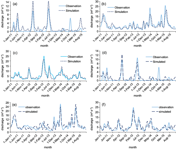
Fig. 5 Comparison of observed and simulated discharge for the validation period using the SWAT model (at monthly time steps): (a) Jazmurian, (b) Khorramabad, and (c) Talar; and the IHACRES model: (d) Jazmurian, (e) Khorramabad, and (f) Talar.
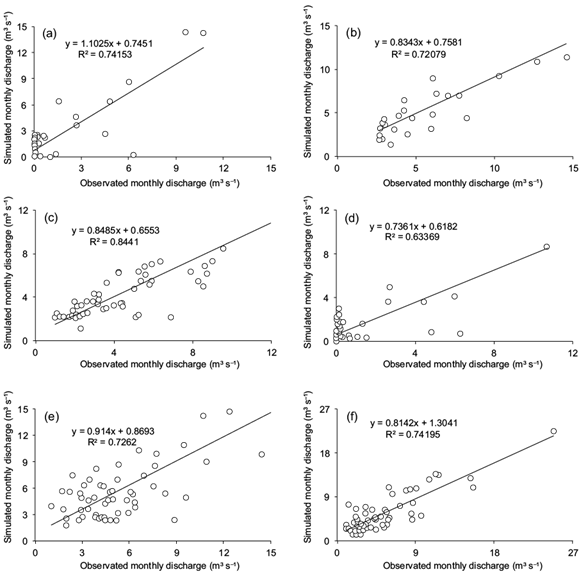
Fig. 6 Correlation between observed and simulated discharge in the validation period using the SWAT model: (a) Jazmurian, (b) Khorramabad, and (c) Talar; and the IHACRES model: (d) Jazmurian, (e) Khorramabad, and (f) Talar.
Table VIII Assessment of the SWAT and IHACRES models performance during the validation period.
| r-factor | p-factor | Dv (%) | PBIAS | NS | R2 | Catchment | Model |
| 0.64 | 0.77 | 11.38 | 5.29 | 0.69 | 0.74 | W arid | SWAT |
| 0.58 | 0.73 | 6.03 | 3.44 | 0.70 | 0.72 | W sa | |
| 0.53 | 0.69 | 4.62 | 4.21 | 0.83 | 0.84 | W sh | |
| - | - | 13.57 | 6.28 | 0.61 | 0.63 | W arid | IHACRES |
| - | - | 12.63 | 5.89 | 0.69 | 0.72 | W sa | |
| - | - | 5.13 | 4.59 | 0.72 | 0.74 | W sh |
5. Conclusions
SWAT and IHACRES are two of the most common models employed in simulating streamflow conditions. In the present study, the simulation of streamflow variation by both models represented a new attempt to estimate hydrological response under different climates. A different condition in each watershed, especially with respect to climate, makes the choice of the appropriate model particularly important. In order to assess the efficacy of the models, three watersheds were selected in different geographic and climatic regions: the Jazmurian watershed in the central part of the country, with an arid climate (W arid ); the Khorramabad watershed in the west, with a semi-arid climate (W sa ); and the Talar watershed in the northern portion of Iran, with a semi-humid climate (W sh ). The models were calibrated and validated for the 2000-2010 and 2011-2015 time periods, respectively. Based on NS, R2, PBIAS, and Dv, the streamflow simulated by these models was assessed.
Both models satisfactorily simulated runoff patterns in time and magnitude. In the arid climate, with 150 mm annual precipitation, IHACRES showed a poorer performance (overestimation) in simulating discharge compared to the SWAT model. In the semi-arid and semi-humid watersheds, with 405- and 610-mm annual precipitation, respectively, the simulated streamflow by both models returned high NS and R2 coefficients, suggesting very good performance. The accuracy of the SWAT model in all the study watersheds was greater than that of the IHACRES model for both calibration and validation periods. The SWAT model uses many parameters and detailed input data which improve the simulation precision. In simulating the runoff, SWAT evaluates the effect of underground water and management activity, which could be very important. However, the results of the IHACRES model showed that it can be used for the study of watersheds, but given its better performance in wetter watersheds, it is suggested that this model be used predominantly in this environment in Iran.

